HI6007 Statistics for Business Decisions: Detailed Solution

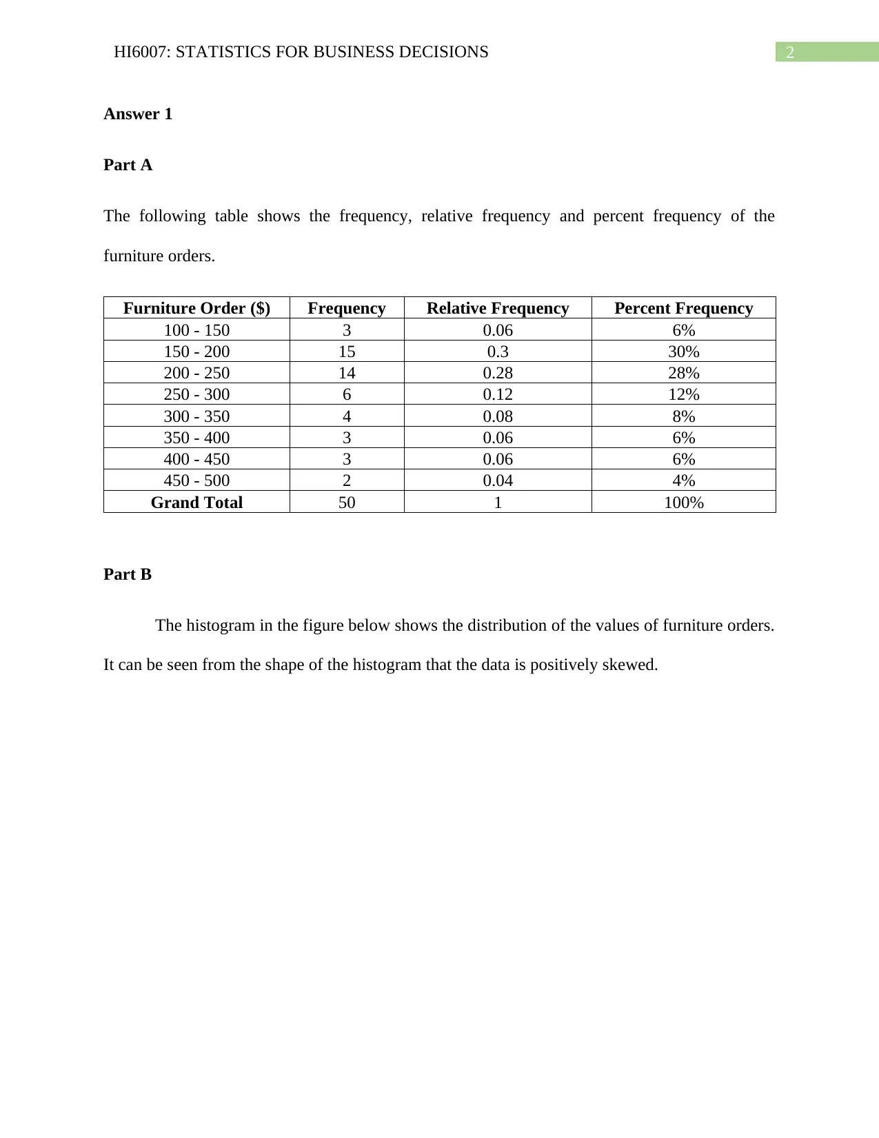
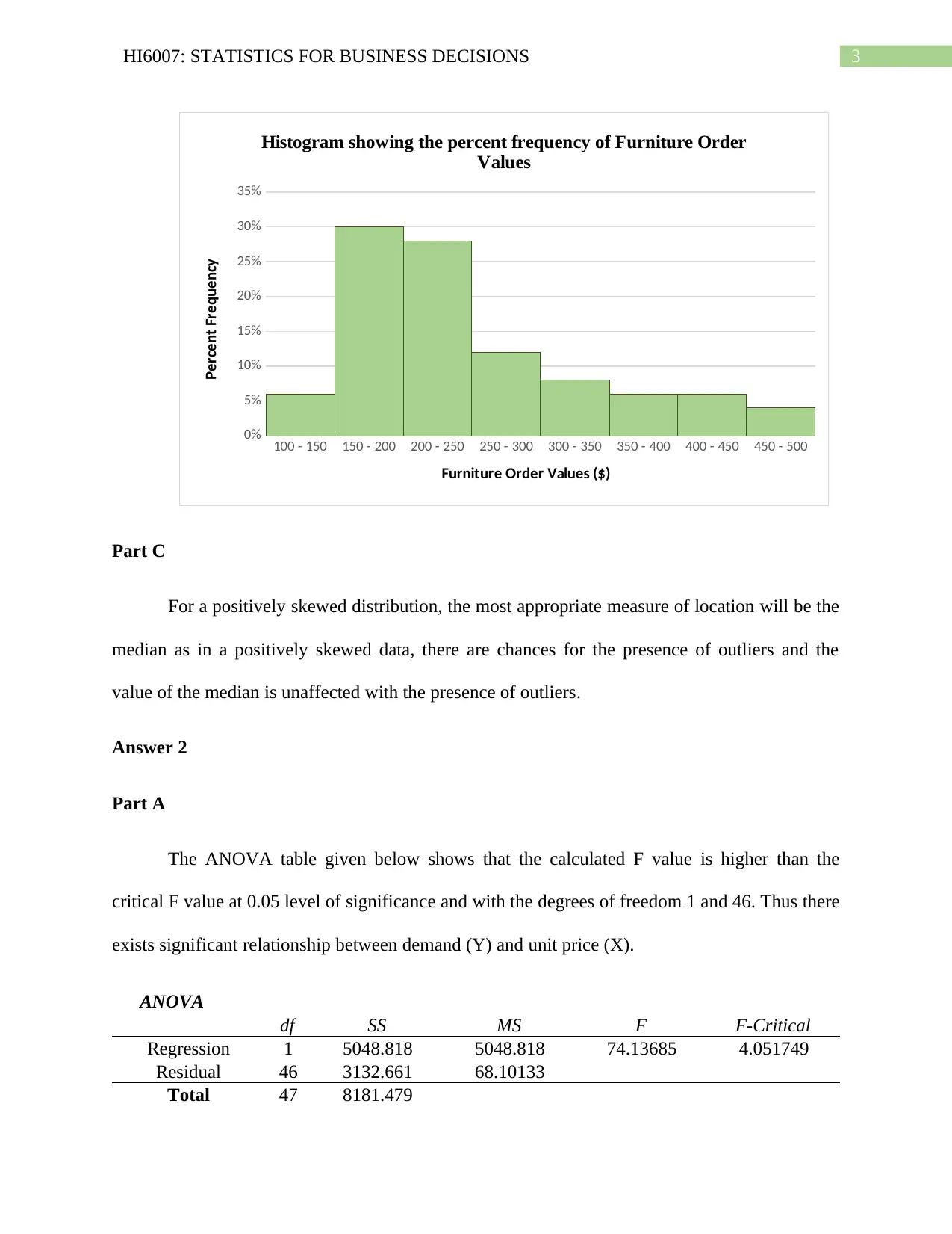
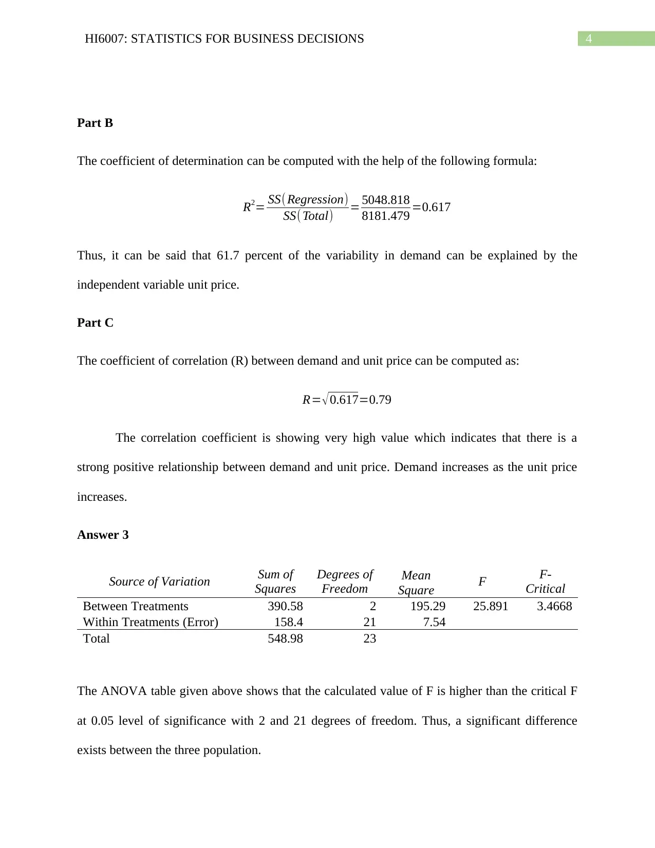
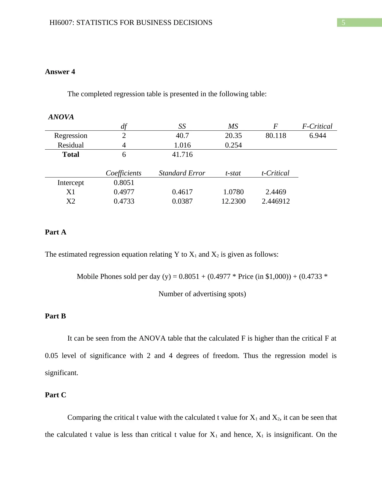
This assignment solution for HI6007 Statistics for Business Decisions addresses several statistical problems. It includes creating frequency, relative frequency, and percent frequency distributions for furniture order data, followed by histogram analysis to determine data skewness and appropriate measures of location. The solution also provides an ANOVA table analysis to determine the relationship between demand and unit price, calculating the coefficient of determination and correlation. Furthermore, it includes completing an ANOVA table and interpreting regression results to assess the significance of variables in a mobile phone sales model, including predicting sales based on price and advertising spots. Desklib offers this solution as a study aid, along with a variety of other solved assignments and past papers to support student learning.

Running Head: HI6007: STATISTICS FOR BUSINESS DECISIONS
HI6007: Statistics For Business Decisions
Name of the Student
Name of the University
Student ID

1HI6007: STATISTICS FOR BUSINESS DECISIONS
Table of Contents
Answer 1..........................................................................................................................................2
Part A...........................................................................................................................................2
Part B...........................................................................................................................................2
Part C...........................................................................................................................................3
Answer 2..........................................................................................................................................3
Part A...........................................................................................................................................3
Part B...........................................................................................................................................4
Part C...........................................................................................................................................4
Answer 3..........................................................................................................................................4
Answer 4..........................................................................................................................................5
Part A...........................................................................................................................................5
Part B...........................................................................................................................................5
Part C...........................................................................................................................................5
Part D...........................................................................................................................................6
Part E...........................................................................................................................................6

2HI6007: STATISTICS FOR BUSINESS DECISIONS
Answer 1
Part A
The following table shows the frequency, relative frequency and percent frequency of the
furniture orders.
Furniture Order ($) Frequency Relative Frequency Percent Frequency
100 - 150 3 0.06 6%
150 - 200 15 0.3 30%
200 - 250 14 0.28 28%
250 - 300 6 0.12 12%
300 - 350 4 0.08 8%
350 - 400 3 0.06 6%
400 - 450 3 0.06 6%
450 - 500 2 0.04 4%
Grand Total 50 1 100%
Part B
The histogram in the figure below shows the distribution of the values of furniture orders.
It can be seen from the shape of the histogram that the data is positively skewed.

3HI6007: STATISTICS FOR BUSINESS DECISIONS
100 - 150 150 - 200 200 - 250 250 - 300 300 - 350 350 - 400 400 - 450 450 - 500
0%
5%
10%
15%
20%
25%
30%
35%
Histogram showing the percent frequency of Furniture Order
Values
Furniture Order Values ($)
Percent Frequency
Part C
For a positively skewed distribution, the most appropriate measure of location will be the
median as in a positively skewed data, there are chances for the presence of outliers and the
value of the median is unaffected with the presence of outliers.
Answer 2
Part A
The ANOVA table given below shows that the calculated F value is higher than the
critical F value at 0.05 level of significance and with the degrees of freedom 1 and 46. Thus there
exists significant relationship between demand (Y) and unit price (X).
ANOVA
df SS MS F F-Critical
Regression 1 5048.818 5048.818 74.13685 4.051749
Residual 46 3132.661 68.10133
Total 47 8181.479

4HI6007: STATISTICS FOR BUSINESS DECISIONS
Part B
The coefficient of determination can be computed with the help of the following formula:
R2= SS( Regression)
SS(Total) = 5048.818
8181.479 =0.617
Thus, it can be said that 61.7 percent of the variability in demand can be explained by the
independent variable unit price.
Part C
The coefficient of correlation (R) between demand and unit price can be computed as:
R= √ 0.617=0.79
The correlation coefficient is showing very high value which indicates that there is a
strong positive relationship between demand and unit price. Demand increases as the unit price
increases.
Answer 3
Source of Variation Sum of
Squares
Degrees of
Freedom
Mean
Square F F-
Critical
Between Treatments 390.58 2 195.29 25.891 3.4668
Within Treatments (Error) 158.4 21 7.54
Total 548.98 23
The ANOVA table given above shows that the calculated value of F is higher than the critical F
at 0.05 level of significance with 2 and 21 degrees of freedom. Thus, a significant difference
exists between the three population.

5HI6007: STATISTICS FOR BUSINESS DECISIONS
Answer 4
The completed regression table is presented in the following table:
ANOVA
df SS MS F F-Critical
Regression 2 40.7 20.35 80.118 6.944
Residual 4 1.016 0.254
Total 6 41.716
Coefficients Standard Error t-stat t-Critical
Intercept 0.8051
X1 0.4977 0.4617 1.0780 2.4469
X2 0.4733 0.0387 12.2300 2.446912
Part A
The estimated regression equation relating Y to X1 and X2 is given as follows:
Mobile Phones sold per day (y) = 0.8051 + (0.4977 * Price (in $1,000)) + (0.4733 *
Number of advertising spots)
Part B
It can be seen from the ANOVA table that the calculated F is higher than the critical F at
0.05 level of significance with 2 and 4 degrees of freedom. Thus the regression model is
significant.
Part C
Comparing the critical t value with the calculated t value for X1 and X2, it can be seen that
the calculated t value is less than critical t value for X1 and hence, X1 is insignificant. On the

6HI6007: STATISTICS FOR BUSINESS DECISIONS
other hand, the calculated t value is more than critical t value for X2 and hence, X2 is significant.
Thus, the coefficient of X2 is significantly different from zero.
Part D
The slope coefficient of X2 (0.4733) indicates that, with each unit increase in the number
of advertising spots, the number of mobile phones sold per day increases by 0.4733.
Part E
If the company charges $20,000 for each phone and uses 10 advertising spots, then the
number of mobile phones that is expected to be sold in a day is given by:
Mobile Phones sold per day (y) = 0.8051 + (0.4977 * 20) + (0.4733 * 10) = 15.49 ~ 16.
Thus, 16 mobile phones can be sold in a day.