HI6007 Statistics Assignment: Statistical Analysis and Interpretation

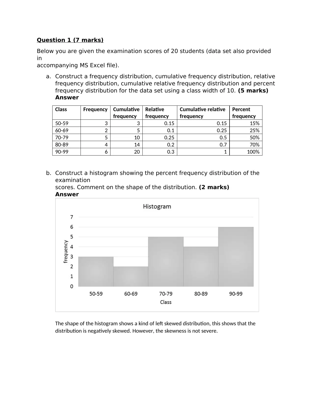
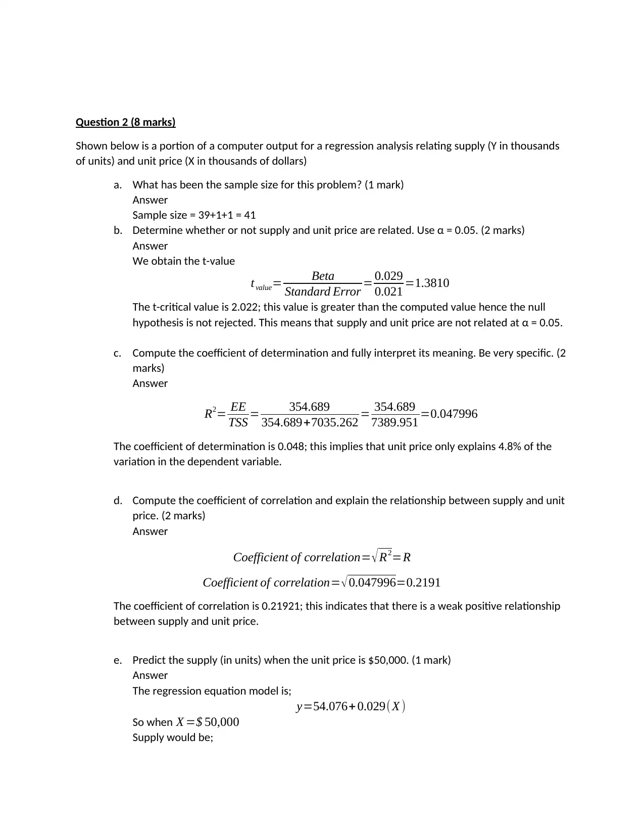
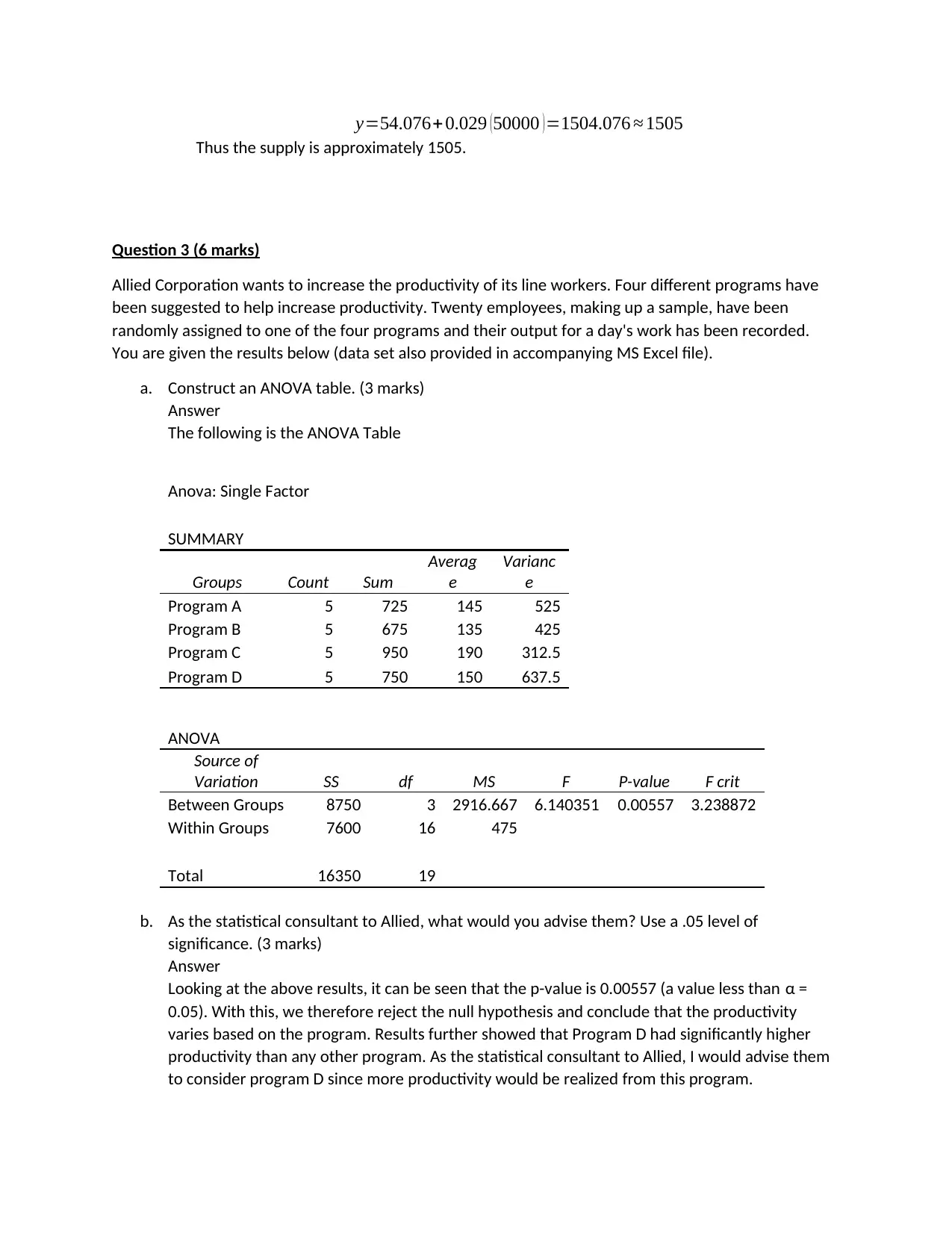
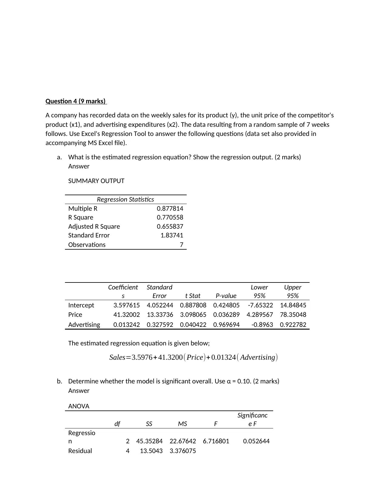
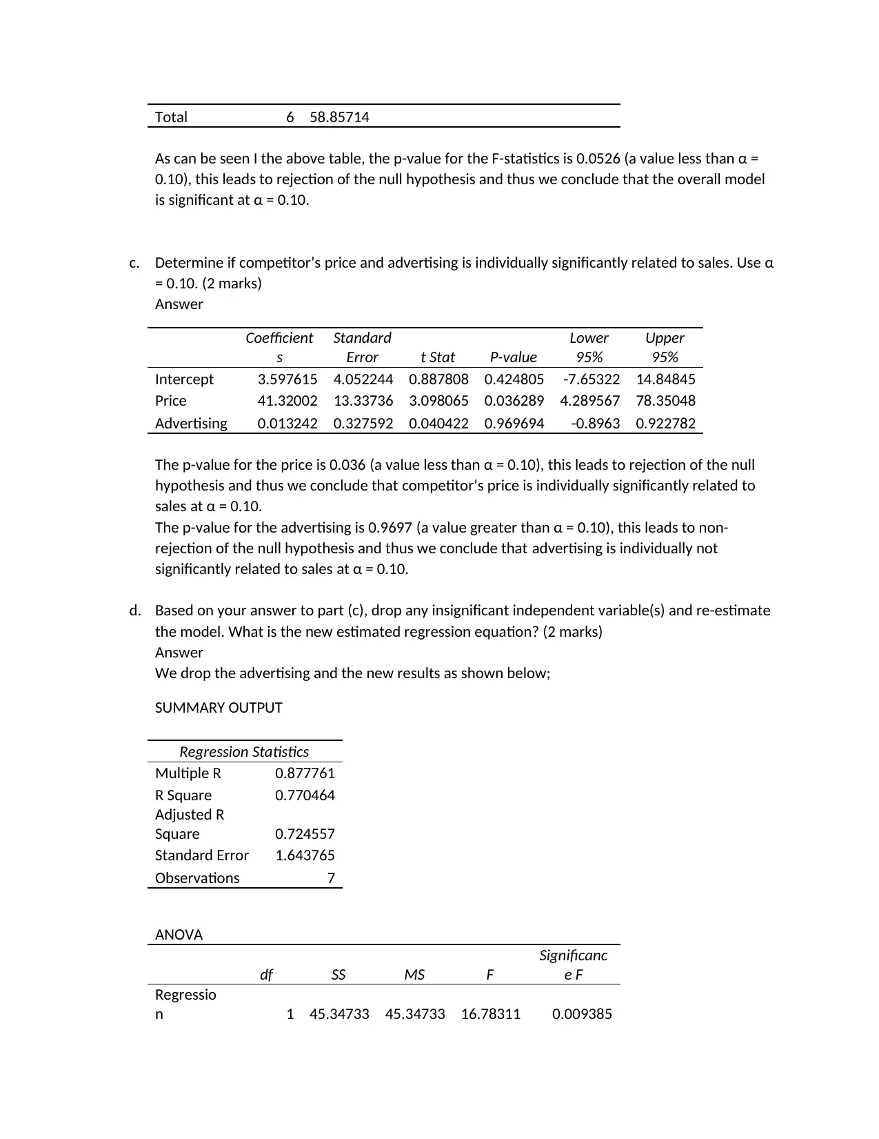
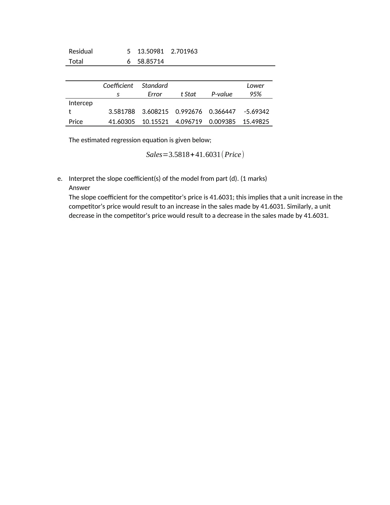
This document presents a complete solution to a statistics assignment for the HI6007 course at Holmes Institute. The assignment covers several key statistical concepts, including the construction of frequency distributions (frequency, cumulative frequency, relative frequency, cumulative relative frequency, and percent frequency), and the creation of histograms to analyze data distributions. It also addresses regression analysis, requiring the interpretation of computer output, hypothesis testing, calculation and interpretation of the coefficient of determination and correlation, and prediction of values. Furthermore, the assignment includes an analysis of variance (ANOVA) problem, involving the construction of an ANOVA table and interpretation of the results to advise on productivity improvement programs. The final part of the assignment involves multiple regression analysis, interpreting regression equations, and determining the significance of variables.

Statistics
Student Name:
Instructor Name:
Course Number:
25 September 2018

Question 1 (7 marks)
Below you are given the examination scores of 20 students (data set also provided
in
accompanying MS Excel file).
a. Construct a frequency distribution, cumulative frequency distribution, relative
frequency distribution, cumulative relative frequency distribution and percent
frequency distribution for the data set using a class width of 10. (5 marks)
Answer
Class Frequency Cumulative
frequency
Relative
frequency
Cumulative relative
frequency
Percent
frequency
50-59 3 3 0.15 0.15 15%
60-69 2 5 0.1 0.25 25%
70-79 5 10 0.25 0.5 50%
80-89 4 14 0.2 0.7 70%
90-99 6 20 0.3 1 100%
b. Construct a histogram showing the percent frequency distribution of the
examination
scores. Comment on the shape of the distribution. (2 marks)
Answer
The shape of the histogram shows a kind of left skewed distribution, this shows that the
distribution is negatively skewed. However, the skewness is not severe.

Question 2 (8 marks)
Shown below is a portion of a computer output for a regression analysis relating supply (Y in thousands
of units) and unit price (X in thousands of dollars)
a. What has been the sample size for this problem? (1 mark)
Answer
Sample size = 39+1+1 = 41
b. Determine whether or not supply and unit price are related. Use α = 0.05. (2 marks)
Answer
We obtain the t-value
tvalue= Beta
Standard Error = 0.029
0.021 =1.3810
The t-critical value is 2.022; this value is greater than the computed value hence the null
hypothesis is not rejected. This means that supply and unit price are not related at α = 0.05.
c. Compute the coefficient of determination and fully interpret its meaning. Be very specific. (2
marks)
Answer
R2= EE
TSS = 354.689
354.689+7035.262 = 354.689
7389.951 =0.047996
The coefficient of determination is 0.048; this implies that unit price only explains 4.8% of the
variation in the dependent variable.
d. Compute the coefficient of correlation and explain the relationship between supply and unit
price. (2 marks)
Answer
Coefficient of correlation= √ R2=R
Coefficient of correlation= √ 0.047996=0.2191
The coefficient of correlation is 0.21921; this indicates that there is a weak positive relationship
between supply and unit price.
e. Predict the supply (in units) when the unit price is $50,000. (1 mark)
Answer
The regression equation model is;
y=54.076+ 0.029(X )
So when X =$ 50,000
Supply would be;

y=54.076+ 0.029 (50000 )=1504.076 ≈ 1505
Thus the supply is approximately 1505.
Question 3 (6 marks)
Allied Corporation wants to increase the productivity of its line workers. Four different programs have
been suggested to help increase productivity. Twenty employees, making up a sample, have been
randomly assigned to one of the four programs and their output for a day's work has been recorded.
You are given the results below (data set also provided in accompanying MS Excel file).
a. Construct an ANOVA table. (3 marks)
Answer
The following is the ANOVA Table
Anova: Single Factor
SUMMARY
Groups Count Sum
Averag
e
Varianc
e
Program A 5 725 145 525
Program B 5 675 135 425
Program C 5 950 190 312.5
Program D 5 750 150 637.5
ANOVA
Source of
Variation SS df MS F P-value F crit
Between Groups 8750 3 2916.667 6.140351 0.00557 3.238872
Within Groups 7600 16 475
Total 16350 19
b. As the statistical consultant to Allied, what would you advise them? Use a .05 level of
significance. (3 marks)
Answer
Looking at the above results, it can be seen that the p-value is 0.00557 (a value less than α =
0.05). With this, we therefore reject the null hypothesis and conclude that the productivity
varies based on the program. Results further showed that Program D had significantly higher
productivity than any other program. As the statistical consultant to Allied, I would advise them
to consider program D since more productivity would be realized from this program.

Question 4 (9 marks)
A company has recorded data on the weekly sales for its product (y), the unit price of the competitor's
product (x1), and advertising expenditures (x2). The data resulting from a random sample of 7 weeks
follows. Use Excel's Regression Tool to answer the following questions (data set also provided in
accompanying MS Excel file).
a. What is the estimated regression equation? Show the regression output. (2 marks)
Answer
SUMMARY OUTPUT
Regression Statistics
Multiple R 0.877814
R Square 0.770558
Adjusted R Square 0.655837
Standard Error 1.83741
Observations 7
Coefficient
s
Standard
Error t Stat P-value
Lower
95%
Upper
95%
Intercept 3.597615 4.052244 0.887808 0.424805 -7.65322 14.84845
Price 41.32002 13.33736 3.098065 0.036289 4.289567 78.35048
Advertising 0.013242 0.327592 0.040422 0.969694 -0.8963 0.922782
The estimated regression equation is given below;
Sales=3.5976+41.3200( Price)+ 0.01324( Advertising)
b. Determine whether the model is significant overall. Use α = 0.10. (2 marks)
Answer
ANOVA
df SS MS F
Significanc
e F
Regressio
n 2 45.35284 22.67642 6.716801 0.052644
Residual 4 13.5043 3.376075

Total 6 58.85714
As can be seen I the above table, the p-value for the F-statistics is 0.0526 (a value less than α =
0.10), this leads to rejection of the null hypothesis and thus we conclude that the overall model
is significant at α = 0.10.
c. Determine if competitor’s price and advertising is individually significantly related to sales. Use α
= 0.10. (2 marks)
Answer
Coefficient
s
Standard
Error t Stat P-value
Lower
95%
Upper
95%
Intercept 3.597615 4.052244 0.887808 0.424805 -7.65322 14.84845
Price 41.32002 13.33736 3.098065 0.036289 4.289567 78.35048
Advertising 0.013242 0.327592 0.040422 0.969694 -0.8963 0.922782
The p-value for the price is 0.036 (a value less than α = 0.10), this leads to rejection of the null
hypothesis and thus we conclude that competitor’s price is individually significantly related to
sales at α = 0.10.
The p-value for the advertising is 0.9697 (a value greater than α = 0.10), this leads to non-
rejection of the null hypothesis and thus we conclude that advertising is individually not
significantly related to sales at α = 0.10.
d. Based on your answer to part (c), drop any insignificant independent variable(s) and re-estimate
the model. What is the new estimated regression equation? (2 marks)
Answer
We drop the advertising and the new results as shown below;
SUMMARY OUTPUT
Regression Statistics
Multiple R 0.877761
R Square 0.770464
Adjusted R
Square 0.724557
Standard Error 1.643765
Observations 7
ANOVA
df SS MS F
Significanc
e F
Regressio
n 1 45.34733 45.34733 16.78311 0.009385

Residual 5 13.50981 2.701963
Total 6 58.85714
Coefficient
s
Standard
Error t Stat P-value
Lower
95%
Intercep
t 3.581788 3.608215 0.992676 0.366447 -5.69342
Price 41.60305 10.15521 4.096719 0.009385 15.49825
The estimated regression equation is given below;
Sales=3.5818+ 41.6031( Price)
e. Interpret the slope coefficient(s) of the model from part (d). (1 marks)
Answer
The slope coefficient for the competitor’s price is 41.6031; this implies that a unit increase in the
competitor’s price would result to an increase in the sales made by 41.6031. Similarly, a unit
decrease in the competitor’s price would result to a decrease in the sales made by 41.6031.