HI6007: Statistics for Business Decisions - Assignment Solution

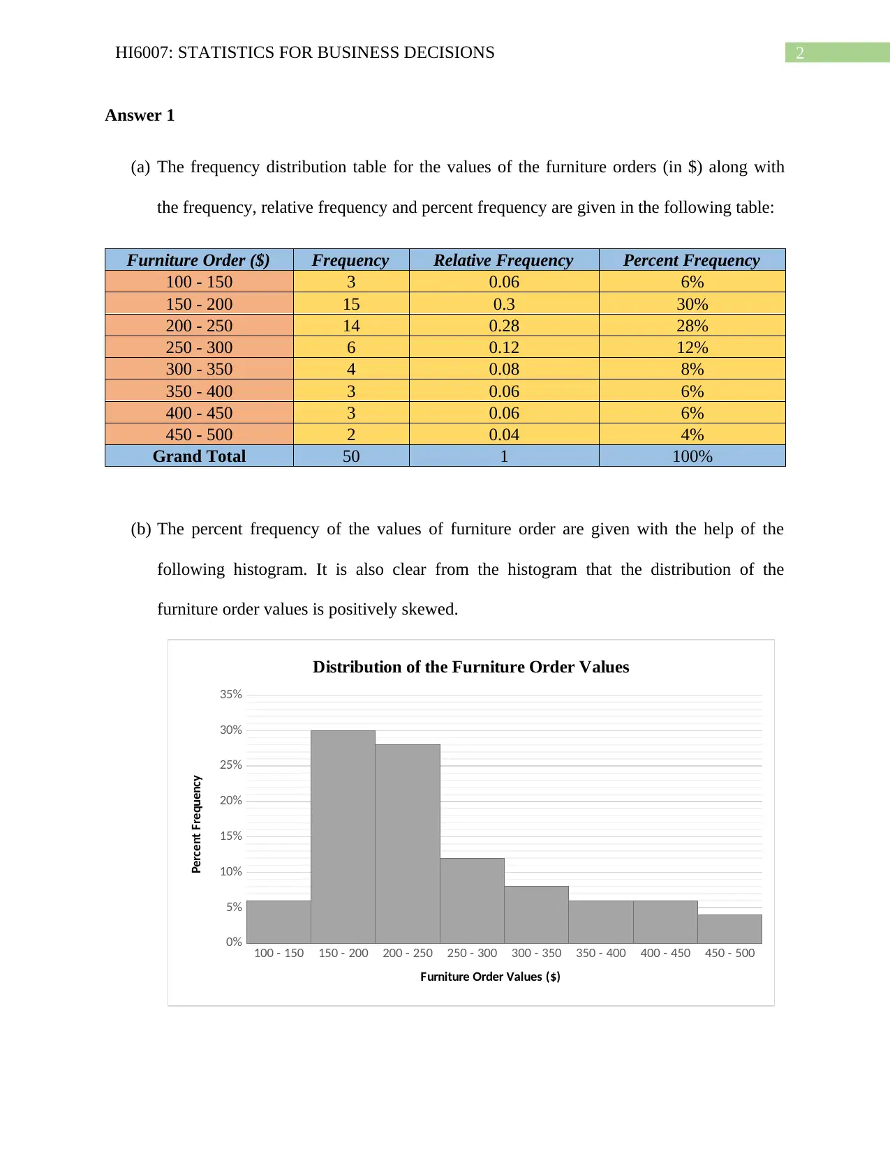
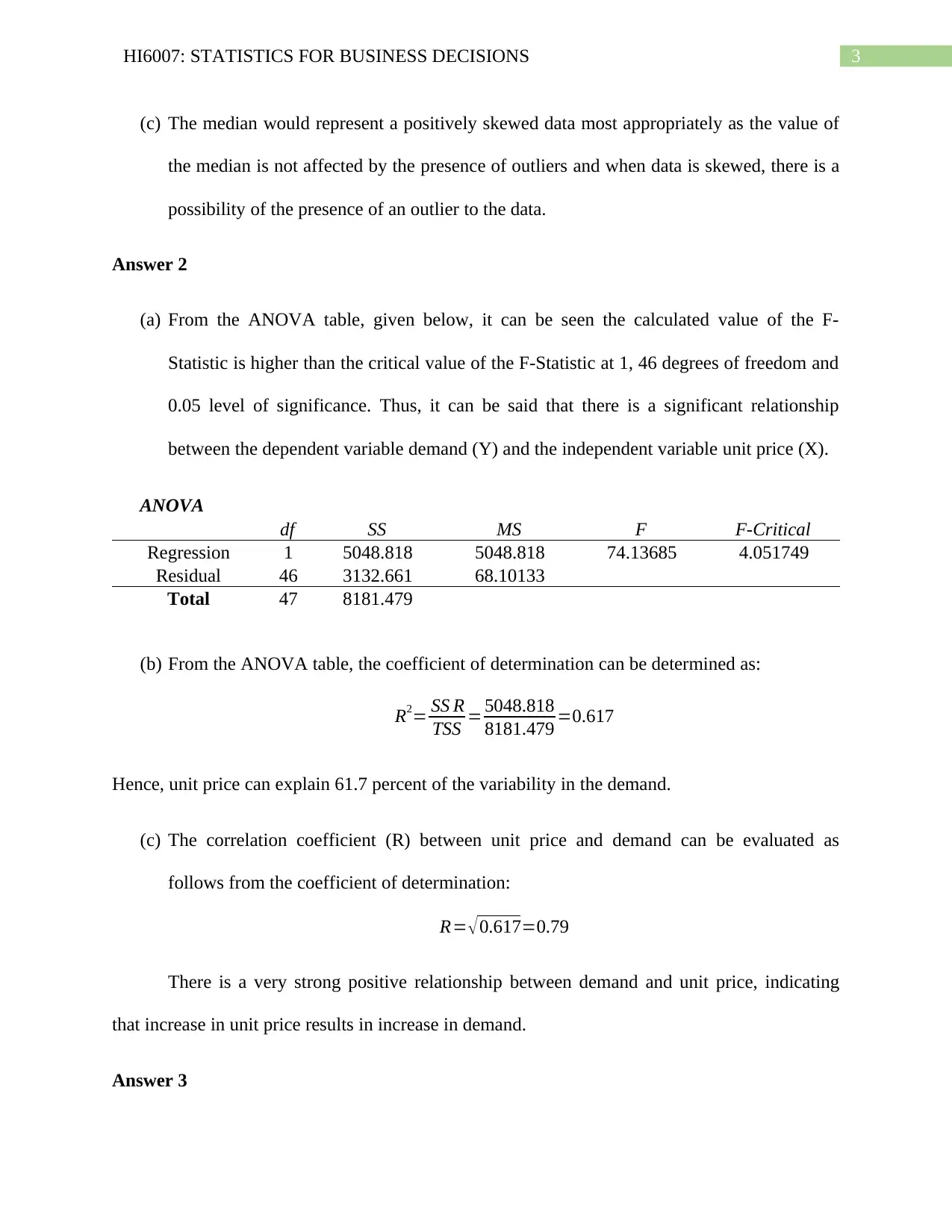
This assignment solution for HI6007 Statistics for Business Decisions covers various statistical concepts and their application in business decision-making. It includes the construction and interpretation of a frequency distribution table and histogram for furniture order values, along with a discussion on the appropriate measure of central tendency for skewed data. The solution also involves ANOVA analysis to determine the relationship between demand and unit price, and to assess the significance of differences between multiple populations. Furthermore, it presents a regression analysis to model the relationship between mobile phone sales, price, and advertising spots, including the interpretation of regression coefficients and hypothesis testing for the significance of independent variables. The assignment uses real-world scenarios to illustrate the practical application of statistical techniques in a business context.

Running Head: HI6007: STATISTICS FOR BUSINESS DECISIONS
HI6007: Statistics For Business Decisions
Name of the Student
Name of the University
Student ID

1HI6007: STATISTICS FOR BUSINESS DECISIONS
Table of Contents
Answer 1..........................................................................................................................................2
Answer 2..........................................................................................................................................3
Answer 3..........................................................................................................................................3
Answer 4..........................................................................................................................................4

2HI6007: STATISTICS FOR BUSINESS DECISIONS
Answer 1
(a) The frequency distribution table for the values of the furniture orders (in $) along with
the frequency, relative frequency and percent frequency are given in the following table:
Furniture Order ($) Frequency Relative Frequency Percent Frequency
100 - 150 3 0.06 6%
150 - 200 15 0.3 30%
200 - 250 14 0.28 28%
250 - 300 6 0.12 12%
300 - 350 4 0.08 8%
350 - 400 3 0.06 6%
400 - 450 3 0.06 6%
450 - 500 2 0.04 4%
Grand Total 50 1 100%
(b) The percent frequency of the values of furniture order are given with the help of the
following histogram. It is also clear from the histogram that the distribution of the
furniture order values is positively skewed.
100 - 150 150 - 200 200 - 250 250 - 300 300 - 350 350 - 400 400 - 450 450 - 500
0%
5%
10%
15%
20%
25%
30%
35%
Distribution of the Furniture Order Values
Furniture Order Values ($)
Percent Frequency

3HI6007: STATISTICS FOR BUSINESS DECISIONS
(c) The median would represent a positively skewed data most appropriately as the value of
the median is not affected by the presence of outliers and when data is skewed, there is a
possibility of the presence of an outlier to the data.
Answer 2
(a) From the ANOVA table, given below, it can be seen the calculated value of the F-
Statistic is higher than the critical value of the F-Statistic at 1, 46 degrees of freedom and
0.05 level of significance. Thus, it can be said that there is a significant relationship
between the dependent variable demand (Y) and the independent variable unit price (X).
ANOVA
df SS MS F F-Critical
Regression 1 5048.818 5048.818 74.13685 4.051749
Residual 46 3132.661 68.10133
Total 47 8181.479
(b) From the ANOVA table, the coefficient of determination can be determined as:
R2= SS R
TSS = 5048.818
8181.479 =0.617
Hence, unit price can explain 61.7 percent of the variability in the demand.
(c) The correlation coefficient (R) between unit price and demand can be evaluated as
follows from the coefficient of determination:
R= √ 0.617=0.79
There is a very strong positive relationship between demand and unit price, indicating
that increase in unit price results in increase in demand.
Answer 3

4HI6007: STATISTICS FOR BUSINESS DECISIONS
Source of Variation Sum of
Squares
Degrees of
Freedom
Mean
Square F F-
Critical
Between Treatments 390.58 2 195.29 25.891 3.4668
Within Treatments (Error) 158.4 21 7.54
Total 548.98 23
From the ANOVA table, given above, it can be seen the calculated value of the F-Statistic is
higher than the critical value of the F-Statistic at 1, 21 degrees of freedom and 0.05 level of
significance. Thus, it can be said that there is a significant difference between the three
populations.
Answer 4
The following table shows the completed ANOVA and Regression table:
ANOVA
df SS MS F F-Critical
Regression 2 40.7 20.35 80.118 6.944
Residual 4 1.016 0.254
Total 6 41.716
Coefficients Standard Error t-stat t-Critical
Intercept 0.8051
X1 0.4977 0.4617 1.0780 2.4469
X2 0.4733 0.0387 12.2300 2.446912
(a) The estimated regression equation of Y (Mobile Phones sold per day) where the
predictors are X1 (Price in $1,000) and X2 (Number of advertising Spots) is given as
follows:
Y = 0.8051 + (0.4977 * X1) + (0.4733 * X2)

5HI6007: STATISTICS FOR BUSINESS DECISIONS
(b) From the ANOVA table, given above, it can be seen the calculated value of the F-
Statistic is higher than the critical value of the F-Statistic at 2, 4 degrees of freedom and
0.05 level of significance. Thus, the developed regression model is significant.
(c) For the variable X1, the calculated value of t-statistic is less than the tabulated t-value.
Thus, X1 is insignificant and the coefficient is not significantly different from zero. On
the other hand, for the variable X2, the calculated value of t-statistic is more than the
tabulated t-value. Thus, X2 is significant and the coefficient is significantly different from
zero.
(d) The slope coefficient of X2 (0.4733) indicates that, with each unit increase in the number
of advertising spots, the number of mobile phones sold per day increases by 0.4733.
(e) If the company charges $20,000 for each phone and uses 10 advertising spots, then the
number of mobile phones that is expected to be sold in a day is given by:
Mobile Phones sold per day (y) = 0.8051 + (0.4977 * 20) + (0.4733 * 10) = 15.49 ~ 16.
Thus, 16 mobile phones can be sold in a day.