HI6007 Statistics Assignment: Regression and Frequency Distribution

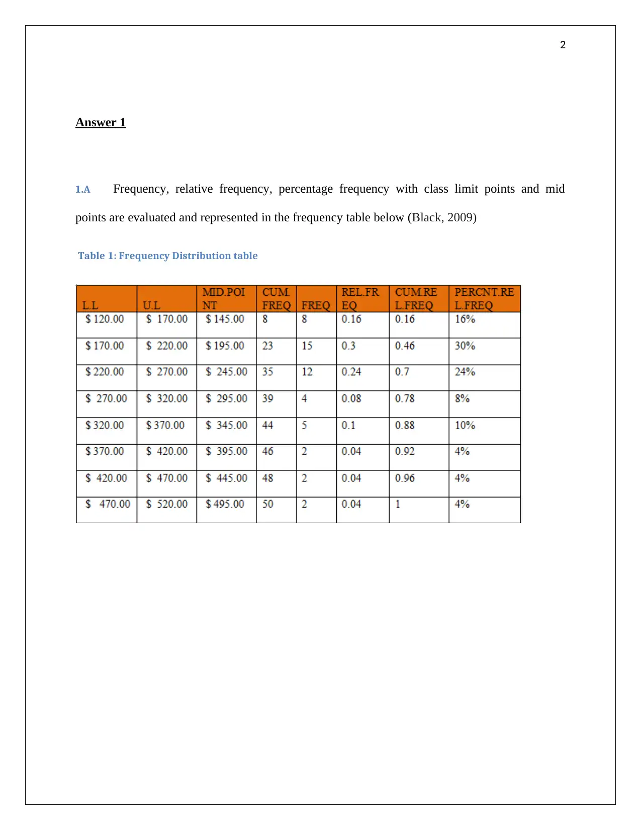
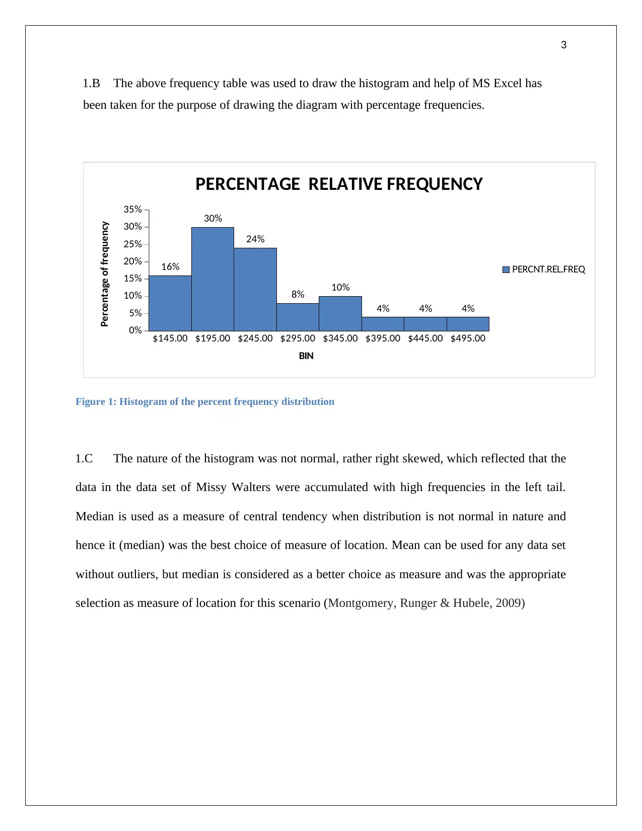
This assignment solution covers several statistical problems. The first problem involves creating a frequency distribution table and histogram from a given dataset, followed by determining the appropriate measure of central tendency. The second problem focuses on regression analysis, deriving a regression equation to model the relationship between demand and unit price, calculating the coefficient of determination, and evaluating the correlation coefficient. The third problem requires completing an ANOVA table and interpreting the results to determine the significance of different treatments. Finally, the fourth problem involves completing ANOVA and regression tables, formulating a regression model, testing hypotheses about the relationships between variables, and predicting mobile phone sales based on price and advertising spots. The solution uses MS Excel for calculations and graphical representations. Desklib offers a wide range of solved assignments and study resources for students.

1
Some Selected Statistical Problems
Student Name: Student ID:
Unit Name: Unit ID:
Date Due: Professor Name:

2
Answer 1
1.A Frequency, relative frequency, percentage frequency with class limit points and mid
points are evaluated and represented in the frequency table below (Black, 2009)
Table 1: Frequency Distribution table

3
1.B The above frequency table was used to draw the histogram and help of MS Excel has
been taken for the purpose of drawing the diagram with percentage frequencies.
$145.00 $195.00 $245.00 $295.00 $345.00 $395.00 $445.00 $495.00
0%
5%
10%
15%
20%
25%
30%
35%
16%
30%
24%
8% 10%
4% 4% 4%
PERCENTAGE RELATIVE FREQUENCY
PERCNT.REL.FREQ
BIN
Percentage of frequency
Figure 1: Histogram of the percent frequency distribution
1.C The nature of the histogram was not normal, rather right skewed, which reflected that the
data in the data set of Missy Walters were accumulated with high frequencies in the left tail.
Median is used as a measure of central tendency when distribution is not normal in nature and
hence it (median) was the best choice of measure of location. Mean can be used for any data set
without outliers, but median is considered as a better choice as measure and was the appropriate
selection as measure of location for this scenario (Montgomery, Runger & Hubele, 2009)

4
Answer 2
2.A The regression equation was Y (demand ) = −2. 137∗X ( unit price) +80 . 39
The predictive model between demand and unit sale price was obtained from the above ANOVA
and regression table. Due to increase in one unit price, it was noticed that demand abridged by
2.14 units, in the regression model. The adverse relation of demand and unit price was earlier
explained by Economic theories.
2.B Coefficient of determination was known to be R2=1− SSE
SST and was calculated
accordingly. The completed ANOVA table was used, where SSE = 3132.66, SST = 8181.48,
R2=1− SSE
SST =1−3132 .66
8181 . 48 =1−0 . 38=0 . 62
It was inferred that unit price was an independent variable and was able to explain 62.0%
variance of the dependent variable (demand).
2.C The evaluation of the correlation coefficient was obvious and calculated as
R=± √ 0 . 62=−0. 79 , it is to be noted that the negative sign was used, as the correlation
coefficient and regression coefficient were considered of same sign .The correlation coefficient
defined that there was statistically significant correlation between unit price and demand. The
nature of the association was highly negative where unit price was a significant factor in
measuring demand of an article.

5
Answer 3
3.A Calculations were done to fill up the blank spaces in the ANOVA table using MS Excel
as provided underneath.
Table 2: ANOVA Table for three treatments
Source of
variation
Sum of
squares
Degrees
of
freedom
Mean
square
F p
Between
Treatments
390.58 2 195.29 25.89 0.00
Within
Treatments
(Error)
158.4 21 7.54
Total 548.98 23 202.83
The given values of SSE, SSB and SST were used for further calculations where degrees of
freedom total was 11. For existence of three treatments m = 3, and for 24 observations n = 24.
Therefore the total degree of freedom was n-1 = 23. Therefore the values were, SSE = 158.4,
SSB = 390.58, SST = 548.98. Consequently calculated values were, MSB = SSB/ (m-1)
=390.58/ 2 =195.29, MSE = SSE/ (n-m) = 158.4/ 21 =7.54, F = MSB / MSE = 195.29/ 7.54 =
25.89. The conforming significance level was less than 0.05 and it was observed that the
outcome was significant at α=0 . 5 level of significance. The F value was 25.89 which at

6
α=0 . 5 was in the critical region. Consequently the null hypothesis considering the three
treatments to be equally effective was rejected (Heiberger & Neuwirth, 2009)
Answer 4
The ANOVA and Regression tables were completed using MS Excel as follows.
Table 3: ANOVA and Regression Data
The calculations used to complete the incomplete tables have been given below:
Total observations was, N = 7, consequently total degree of freedom was, N – 1 = 6. Existence of
two independent variables indicated degrees of freedom for regression as 2, for residual DF was
4 (6 – 2 = 4). Currently, SSB = 40.7 and SSE = 1.016, so SST = (40.7 + 1.016) = 41.716. MSB =
SSB /2 = 20.35, MSE = SSE/ 4 = 0.254. MST = MSB + MSE. The calculation of F value was
done as the ratio between MSB and MSE. Significant value was evaluated using the F-
distribution function (Albright, Winston & Zappe, 2010).
Standard error of intercept in regression analysis was found as
SEslope= √ SSE /(n−2 )
√ SST and t-
values were calculated as the proportion of coefficients and standard errors. The p-values were
found using the t-distribution function.

7
4.A Using the completed regression table, the estimated regression model was evaluated as
Y =0 . 8051+0 . 4977 X1+ 0. 4733 X2
4.B The null hypothesis: H0: There was no significant relation between mobiles sold and the
independent factors, price and advertising spots.
4.C The alternate hypothesis: HA: There was significant relation between mobiles sold and
the independent factors, price and advertising spots.
Using the Regression table t-values for X1 and X2 variables were 1.08 (with p-value = 0.33)
and 12.23 (with p-value < 0.05), it was apparent that variable X1 did not have significant
correlation with number of phones sold per day (Y). Therefore, the estimated regression model
was not statistically significant (Draper & Smith, 2014).
4.D For the validity of association of the two regression coefficients, hypotheses were tested.
For the coefficient β1, the null hypothesis was: H0: β1 = 0 and alternate hypothesis was: HA:
β1≠0.
The result was estimated using t-test where the statistic was evaluated as
t = 0. 4977−0
0 . 4617 =1 . 08
(with p-value =0.33). Therefore the null hypothesis could not be rejected at α=0 . 5 level of
significance. The first coefficient of price was not significantly different from zero (Cameron &
Trivedi, 2013).
For the coefficient β2, let the null hypothesis was: H0: β2 = 0 and alternate hypothesis: HA:
β2≠0.

8
The result was estimated using t-test where statistic was evaluated as
t = 0. 4733−0
0. 0387 =12 . 23
(with p-value < 0.05). Therefore the null hypothesis was rejected at α =0 . 5 level of
significance. The coefficient was significantly different from zero.
4.E The slope or intercept of the regression model was 0.8051 and the statement was that the
coefficient had positive sign. Therefore it was inferred that mobiles sold per day had a
significant sales figure when the independent influences were kept at zero.
4.F From the regression equation Y =0 . 8051+0 . 4977 X1+ 0. 4733 X2 , taking X1= $20,000
and X2 = 10, Y =0 . 8051+0 . 4977∗20000+0 . 4733∗10=9959 . 5≃9960
Consequently, the predicted transactions of 9960 mobiles were noticed (Seber & Lee, 2012).
.

9
References
Albright, S.C., Winston, W. and Zappe, C., 2010. Data analysis and decision making. Cengage
Learning)
Black, K., 2009. Business statistics: Contemporary decision making. John Wiley & Sons.
Cameron, A.C. and Trivedi, P.K., 2013. Regression analysis of count data (Vol. 53).
Cambridge university press.
Draper, N.R. and Smith, H., 2014. Applied regression analysis (Vol. 326). John Wiley & Sons.
Heiberger, R.M. and Neuwirth, E., 2009. One-way anova. In R through excel (pp. 165-191).
Springer, New York, NY.
Montgomery, D. C., Peck, E. A., & Vining, G. G. (2012). Introduction to linear regression
analysis (Vol. 821). John Wiley & Sons.
Montgomery, D.C., Runger, G.C. and Hubele, N.F., 2009. Engineering statistics. John Wiley &
Sons.
Seber, G.A. and Lee, A.J., 2012. Linear regression analysis (Vol. 329). John Wiley & Sons.