Business Analytics and Statistics Report: Honeybee Fruit Performance

This report presents a comprehensive analysis of Honeybee Fruit's business performance, addressing key challenges related to revenue, cost of goods, and average sales. Using a dataset from the second year of the business, the study investigates several research questions. These include identifying the best and worst-selling products, comparing payment methods (cash vs. credit), examining the impact of product location on sales, analyzing sales and gross profits across different months, and assessing seasonal variations in sales performance. The analysis employs various statistical methods, including frequency statistics, t-tests, and ANOVA. Key findings reveal significant differences in sales between payment methods, with credit sales outperforming cash. Product location also significantly impacts sales, with products located outside the front of the store generating the highest revenue. Furthermore, while there is no significant difference in overall gross sales across different months, there are significant differences in gross profits, particularly between October and March, and October and April. The report concludes with recommendations based on the findings, aiming to support the CEO's decision-making process.

Business Analytics and Statistics
Student Name:
Instructor Name:
Course Number:
18 September 2018

Table of Contents
Introduction......................................................................................................................................2
Problem definition and business intelligence required....................................................................2
Results of the selected analytics methods and technical analysis....................................................4
What are the best and worst selling products in terms of sales?..................................................4
Is there a difference in payments methods? (Cash vs Credit)?....................................................5
Are the differences in sales performance based on where the product is located in the shop?
How does this effect both profits and revenue?...........................................................................5
Is there a difference in sales and gross profits between different months of the year?................7
Are their differences in sales performance between different seasons?......................................9
Discussion of the results and recommendations............................................................................10
Recommendations......................................................................................................................10
References......................................................................................................................................11
Appendix........................................................................................................................................12

List of tables
Table 1: Top best-selling products in terms of sales.......................................................................5
Table 2: Worst selling products in terms of sales............................................................................6
Table 3: t-Test: Two-Sample Assuming Equal Variances..............................................................6
Table 4: Descriptive statistics..........................................................................................................7
Table 5: Test of Homogeneity of Variances....................................................................................7
Table 6: ANOVA.............................................................................................................................8
Table 7: ANOVA.............................................................................................................................8
Table 8: Descriptive Statistics.........................................................................................................9
Table 9: Test of Homogeneity of Variances..................................................................................10
Table 10: ANOVA.........................................................................................................................10
Table 11: Descriptive statistics......................................................................................................11
Table 12: ANOVA.........................................................................................................................11

Introduction
This report sought to present findings to the CEO of Honeybee Fruit in relation to the
performance of the business.
We ae provided with data that is inclusive of a whole year of trading. This is the second
year of business and the business is still in a start-up phase. The reported high Cost of
Goods (COGS) is reportedly consistent with the Organic fruit industry.
The study focusses on the main challenges of the business which are revenue (i.e. lead
generation/new business), Cost of Goods (COGS margins) and average sales. We seek to
answer a number of research questions which at the end would answer the concerns of the
CEO.
Problem definition and business intelligence required
The following are the research questions that this study sought to respond to;
1. What are the best and worst selling products in terms of sales?
For this question, we sought to look at the frequency statistics. We looked at the
measures of central tendency such as the mean, median and the mode to understand the
distribution of the sales data for the various products. This is ideal since we are not
testing any hypothesis but rather trying to figure out how the distribution looks like
(Bonett & Seier, 2006).
2. Is there a difference in payments methods? (Cash vs Credit)
For this question, we sought to compare the mean differences between the two payments
methods (Cash and Credit). As such an ideal test that was to be used was the t-test. T-test
helps test and compare the average differences in two groups and in this case we had two

groups (Cash and Credit) hence the test was the most ideal (Derrick, Broad, Toher, &
White, 2017)
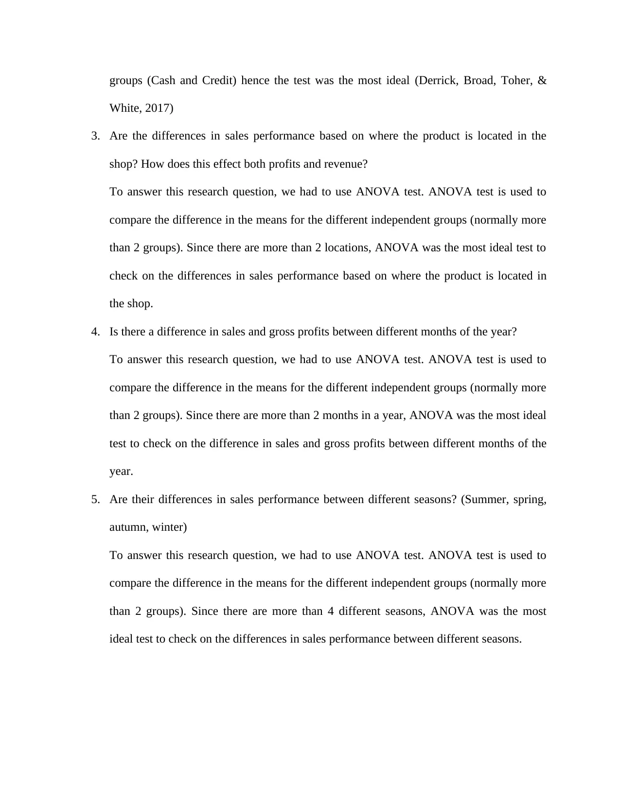
3. Are the differences in sales performance based on where the product is located in the
shop? How does this effect both profits and revenue?
To answer this research question, we had to use ANOVA test. ANOVA test is used to
compare the difference in the means for the different independent groups (normally more
than 2 groups). Since there are more than 2 locations, ANOVA was the most ideal test to
check on the differences in sales performance based on where the product is located in
the shop.
4. Is there a difference in sales and gross profits between different months of the year?
To answer this research question, we had to use ANOVA test. ANOVA test is used to
compare the difference in the means for the different independent groups (normally more
than 2 groups). Since there are more than 2 months in a year, ANOVA was the most ideal
test to check on the difference in sales and gross profits between different months of the
year.
5. Are their differences in sales performance between different seasons? (Summer, spring,
autumn, winter)
To answer this research question, we had to use ANOVA test. ANOVA test is used to
compare the difference in the means for the different independent groups (normally more
than 2 groups). Since there are more than 4 different seasons, ANOVA was the most
ideal test to check on the differences in sales performance between different seasons.

Results of the selected analytics methods and technical analysis
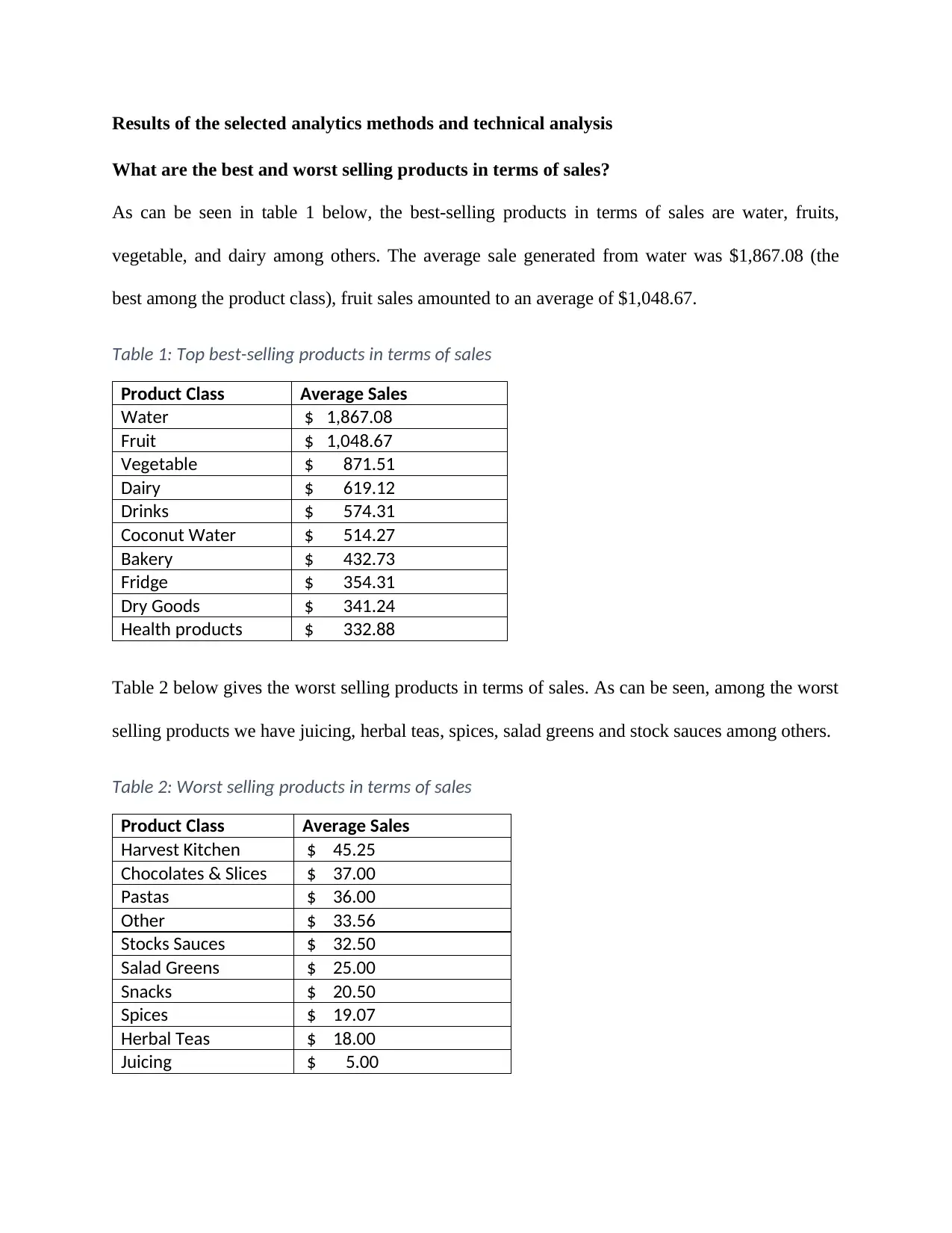
What are the best and worst selling products in terms of sales?
As can be seen in table 1 below, the best-selling products in terms of sales are water, fruits,
vegetable, and dairy among others. The average sale generated from water was $1,867.08 (the
best among the product class), fruit sales amounted to an average of $1,048.67.
Table 1: Top best-selling products in terms of sales
Product Class Average Sales
Water $ 1,867.08
Fruit $ 1,048.67
Vegetable $ 871.51
Dairy $ 619.12
Drinks $ 574.31
Coconut Water $ 514.27
Bakery $ 432.73
Fridge $ 354.31
Dry Goods $ 341.24
Health products $ 332.88
Table 2 below gives the worst selling products in terms of sales. As can be seen, among the worst
selling products we have juicing, herbal teas, spices, salad greens and stock sauces among others.
Table 2: Worst selling products in terms of sales
Product Class Average Sales
Harvest Kitchen $ 45.25
Chocolates & Slices $ 37.00
Pastas $ 36.00
Other $ 33.56
Stocks Sauces $ 32.50
Salad Greens $ 25.00
Snacks $ 20.50
Spices $ 19.07
Herbal Teas $ 18.00
Juicing $ 5.00

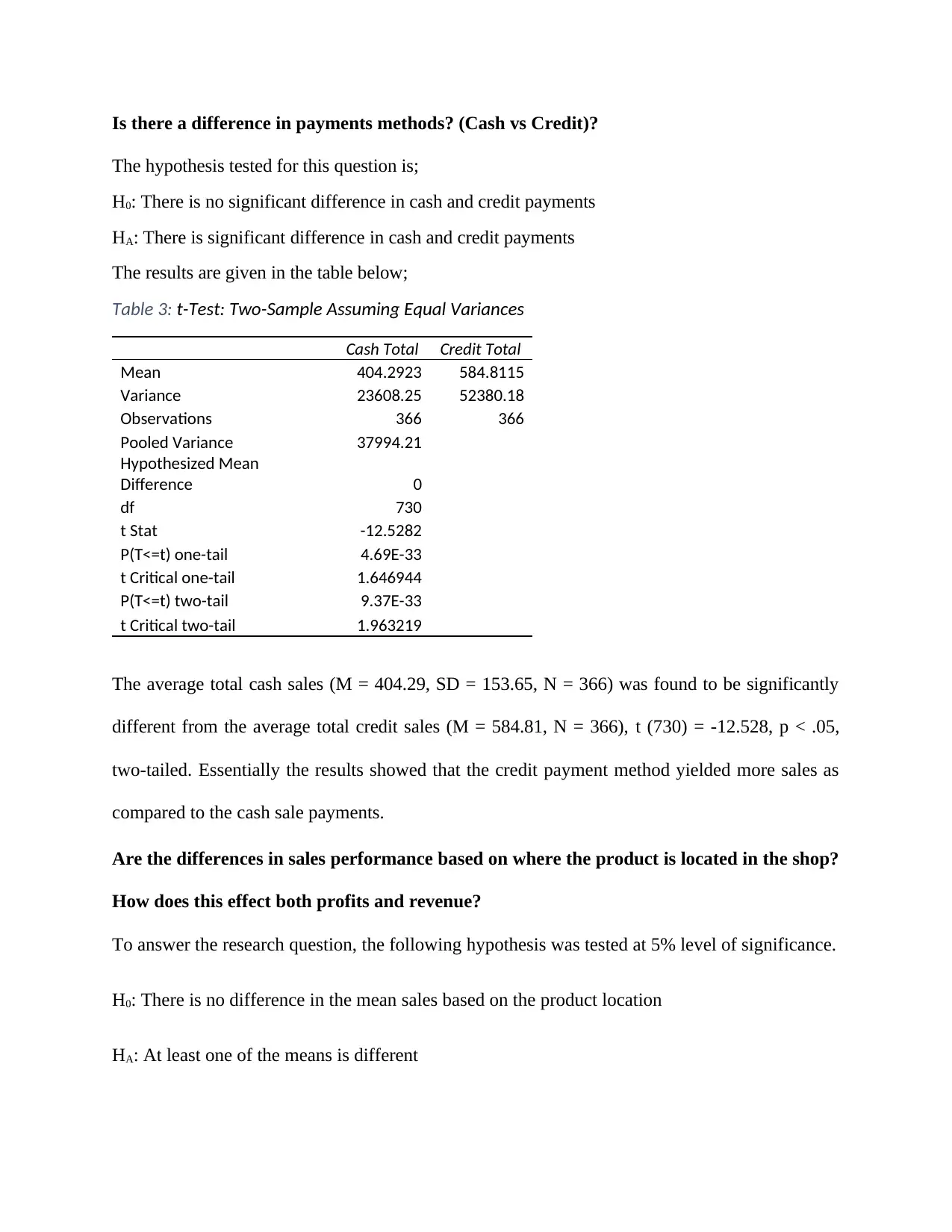
Is there a difference in payments methods? (Cash vs Credit)?
The hypothesis tested for this question is;
H0: There is no significant difference in cash and credit payments
HA: There is significant difference in cash and credit payments
The results are given in the table below;
Table 3: t-Test: Two-Sample Assuming Equal Variances
Cash Total Credit Total
Mean 404.2923 584.8115
Variance 23608.25 52380.18
Observations 366 366
Pooled Variance 37994.21
Hypothesized Mean
Difference 0
df 730
t Stat -12.5282
P(T<=t) one-tail 4.69E-33
t Critical one-tail 1.646944
P(T<=t) two-tail 9.37E-33
t Critical two-tail 1.963219
The average total cash sales (M = 404.29, SD = 153.65, N = 366) was found to be significantly
different from the average total credit sales (M = 584.81, N = 366), t (730) = -12.528, p < .05,
two-tailed. Essentially the results showed that the credit payment method yielded more sales as
compared to the cash sale payments.
Are the differences in sales performance based on where the product is located in the shop?
How does this effect both profits and revenue?
To answer the research question, the following hypothesis was tested at 5% level of significance.
H0: There is no difference in the mean sales based on the product location
HA: At least one of the means is different

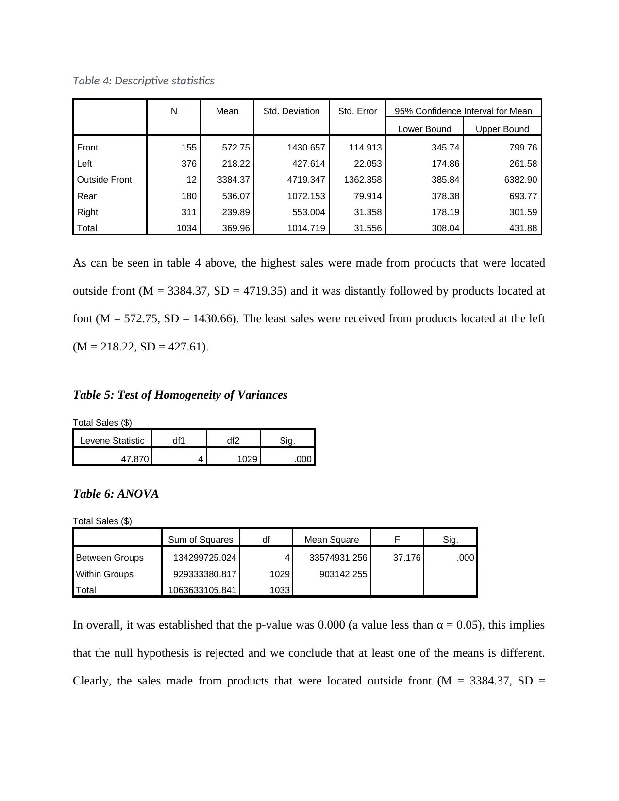
Table 4: Descriptive statistics
N Mean Std. Deviation Std. Error 95% Confidence Interval for Mean
Lower Bound Upper Bound
Front 155 572.75 1430.657 114.913 345.74 799.76
Left 376 218.22 427.614 22.053 174.86 261.58
Outside Front 12 3384.37 4719.347 1362.358 385.84 6382.90
Rear 180 536.07 1072.153 79.914 378.38 693.77
Right 311 239.89 553.004 31.358 178.19 301.59
Total 1034 369.96 1014.719 31.556 308.04 431.88
As can be seen in table 4 above, the highest sales were made from products that were located
outside front (M = 3384.37, SD = 4719.35) and it was distantly followed by products located at
font (M = 572.75, SD = 1430.66). The least sales were received from products located at the left
(M = 218.22, SD = 427.61).
Table 5: Test of Homogeneity of Variances
Total Sales ($)
Levene Statistic df1 df2 Sig.
47.870 4 1029 .000
Table 6: ANOVA
Total Sales ($)
Sum of Squares df Mean Square F Sig.
Between Groups 134299725.024 4 33574931.256 37.176 .000
Within Groups 929333380.817 1029 903142.255
Total 1063633105.841 1033
In overall, it was established that the p-value was 0.000 (a value less than α = 0.05), this implies
that the null hypothesis is rejected and we conclude that at least one of the means is different.
Clearly, the sales made from products that were located outside front (M = 3384.37, SD =

4719.35) were significantly greater than the sales received from products located at front (M =
572.75, SD = 1430.66) and from any other location.
The fact that location of the product significantly affects the sales received will also have some
significant effect on both profits and revenue. Profits and revenues are generated from sales so
whatever affects sales will automatically affect the profits and revenues.
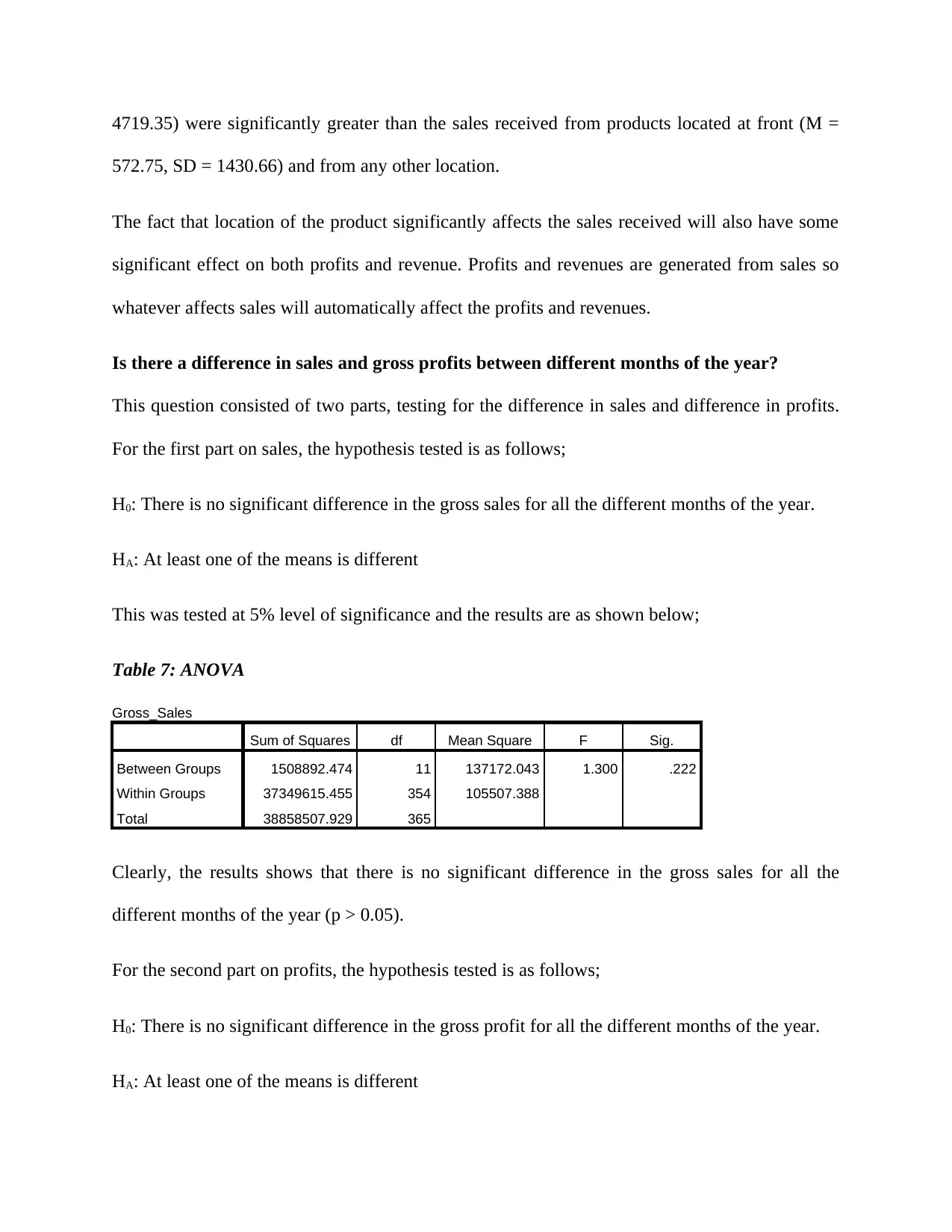
Is there a difference in sales and gross profits between different months of the year?
This question consisted of two parts, testing for the difference in sales and difference in profits.
For the first part on sales, the hypothesis tested is as follows;
H0: There is no significant difference in the gross sales for all the different months of the year.
HA: At least one of the means is different
This was tested at 5% level of significance and the results are as shown below;
Table 7: ANOVA
Gross_Sales
Sum of Squares df Mean Square F Sig.
Between Groups 1508892.474 11 137172.043 1.300 .222
Within Groups 37349615.455 354 105507.388
Total 38858507.929 365
Clearly, the results shows that there is no significant difference in the gross sales for all the
different months of the year (p > 0.05).
For the second part on profits, the hypothesis tested is as follows;
H0: There is no significant difference in the gross profit for all the different months of the year.
HA: At least one of the means is different

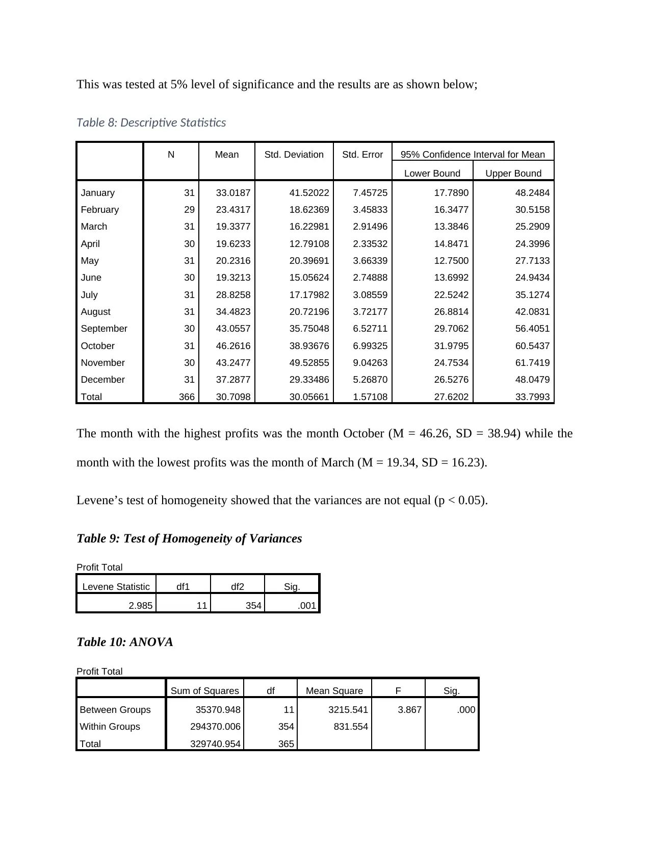
This was tested at 5% level of significance and the results are as shown below;
Table 8: Descriptive Statistics
N Mean Std. Deviation Std. Error 95% Confidence Interval for Mean
Lower Bound Upper Bound
January 31 33.0187 41.52022 7.45725 17.7890 48.2484
February 29 23.4317 18.62369 3.45833 16.3477 30.5158
March 31 19.3377 16.22981 2.91496 13.3846 25.2909
April 30 19.6233 12.79108 2.33532 14.8471 24.3996
May 31 20.2316 20.39691 3.66339 12.7500 27.7133
June 30 19.3213 15.05624 2.74888 13.6992 24.9434
July 31 28.8258 17.17982 3.08559 22.5242 35.1274
August 31 34.4823 20.72196 3.72177 26.8814 42.0831
September 30 43.0557 35.75048 6.52711 29.7062 56.4051
October 31 46.2616 38.93676 6.99325 31.9795 60.5437
November 30 43.2477 49.52855 9.04263 24.7534 61.7419
December 31 37.2877 29.33486 5.26870 26.5276 48.0479
Total 366 30.7098 30.05661 1.57108 27.6202 33.7993
The month with the highest profits was the month October (M = 46.26, SD = 38.94) while the
month with the lowest profits was the month of March (M = 19.34, SD = 16.23).
Levene’s test of homogeneity showed that the variances are not equal (p < 0.05).
Table 9: Test of Homogeneity of Variances
Profit Total
Levene Statistic df1 df2 Sig.
2.985 11 354 .001
Table 10: ANOVA
Profit Total
Sum of Squares df Mean Square F Sig.
Between Groups 35370.948 11 3215.541 3.867 .000
Within Groups 294370.006 354 831.554
Total 329740.954 365

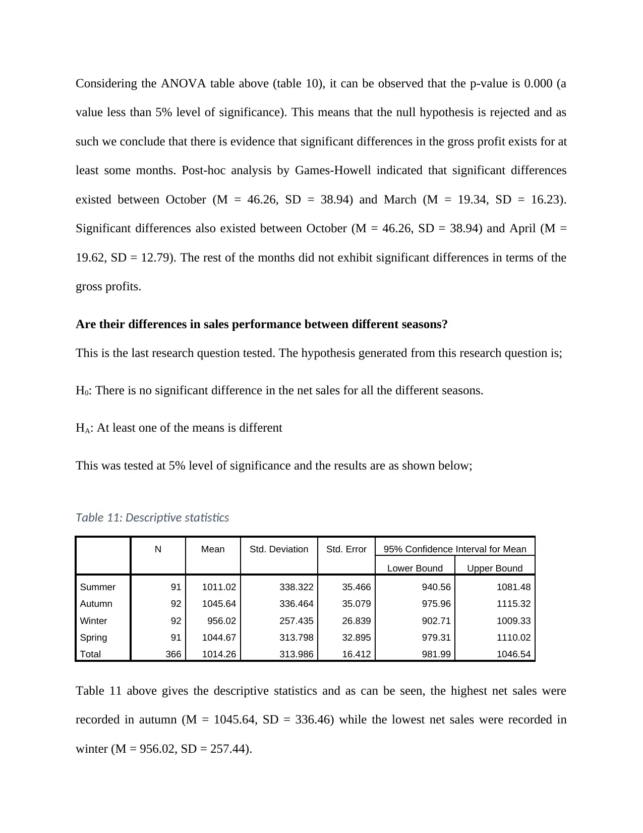
Considering the ANOVA table above (table 10), it can be observed that the p-value is 0.000 (a
value less than 5% level of significance). This means that the null hypothesis is rejected and as
such we conclude that there is evidence that significant differences in the gross profit exists for at
least some months. Post-hoc analysis by Games-Howell indicated that significant differences
existed between October (M = 46.26, SD = 38.94) and March (M = 19.34, SD = 16.23).
Significant differences also existed between October (M = 46.26, SD = 38.94) and April (M =
19.62, SD = 12.79). The rest of the months did not exhibit significant differences in terms of the
gross profits.
Are their differences in sales performance between different seasons?
This is the last research question tested. The hypothesis generated from this research question is;
H0: There is no significant difference in the net sales for all the different seasons.
HA: At least one of the means is different
This was tested at 5% level of significance and the results are as shown below;
Table 11: Descriptive statistics
N Mean Std. Deviation Std. Error 95% Confidence Interval for Mean
Lower Bound Upper Bound
Summer 91 1011.02 338.322 35.466 940.56 1081.48
Autumn 92 1045.64 336.464 35.079 975.96 1115.32
Winter 92 956.02 257.435 26.839 902.71 1009.33
Spring 91 1044.67 313.798 32.895 979.31 1110.02
Total 366 1014.26 313.986 16.412 981.99 1046.54
Table 11 above gives the descriptive statistics and as can be seen, the highest net sales were
recorded in autumn (M = 1045.64, SD = 336.46) while the lowest net sales were recorded in
winter (M = 956.02, SD = 257.44).

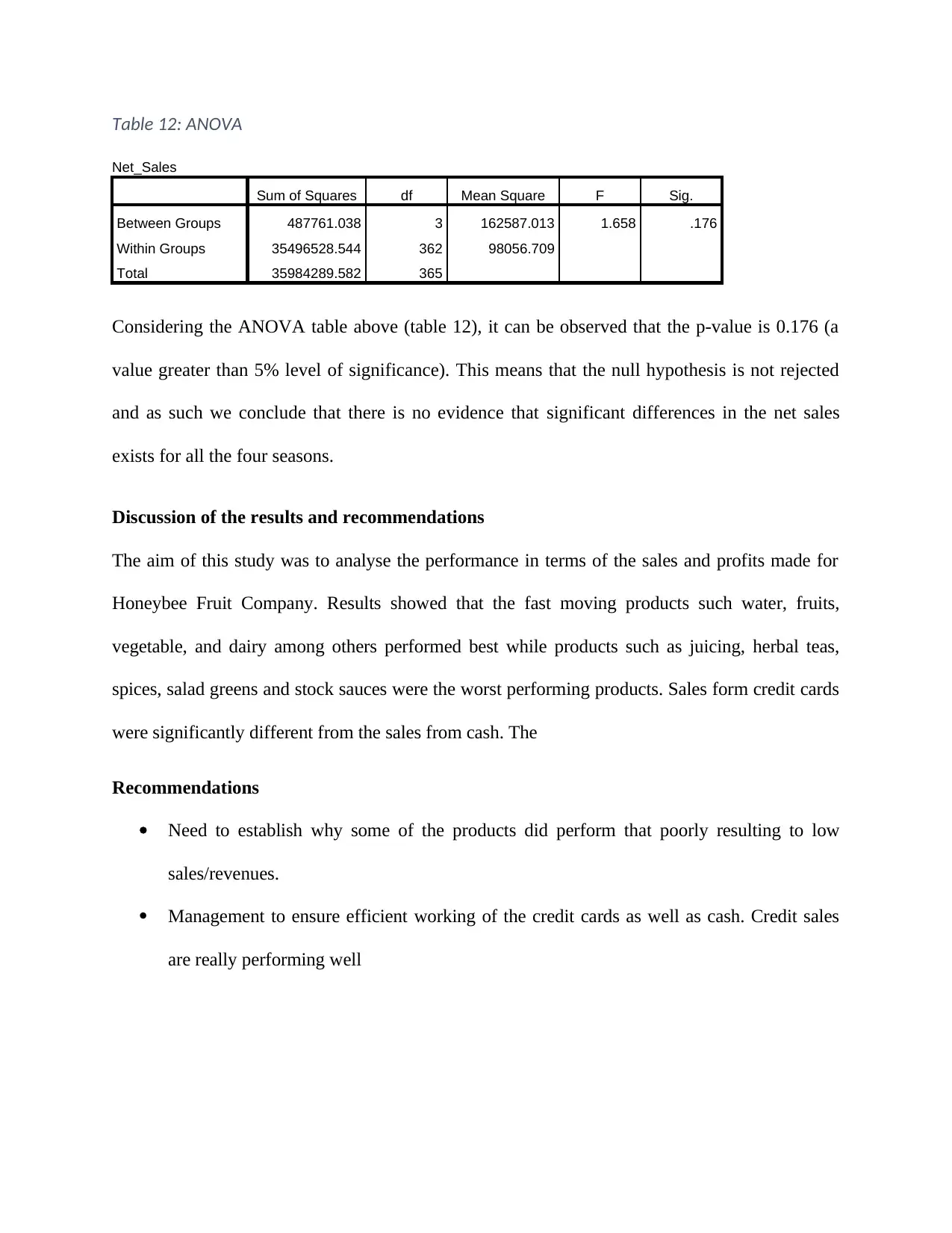
Table 12: ANOVA
Net_Sales
Sum of Squares df Mean Square F Sig.
Between Groups 487761.038 3 162587.013 1.658 .176
Within Groups 35496528.544 362 98056.709
Total 35984289.582 365
Considering the ANOVA table above (table 12), it can be observed that the p-value is 0.176 (a
value greater than 5% level of significance). This means that the null hypothesis is not rejected
and as such we conclude that there is no evidence that significant differences in the net sales
exists for all the four seasons.
Discussion of the results and recommendations
The aim of this study was to analyse the performance in terms of the sales and profits made for
Honeybee Fruit Company. Results showed that the fast moving products such water, fruits,
vegetable, and dairy among others performed best while products such as juicing, herbal teas,
spices, salad greens and stock sauces were the worst performing products. Sales form credit cards
were significantly different from the sales from cash. The
Recommendations
 Need to establish why some of the products did perform that poorly resulting to low
sales/revenues.
 Management to ensure efficient working of the credit cards as well as cash. Credit sales
are really performing well