Planning and Forecasting House Prices: UK Economics & Finance H5
VerifiedAdded on 2023/06/10
|24
|3871
|185
Report
AI Summary
This report analyzes the planning and forecasting of house prices in the UK, focusing on the impact of government subsidies, credit scores, and mortgage rates. It examines the economics of house prices, considering housing as both a consumer good and an investment. The study uses OLS regression and log-linear regression models to estimate the relationship between house prices and factors like gross household income, mortgage rates, and government schemes. The results indicate a significant positive correlation between house prices and gross household income, while the impact of mortgage rates varies depending on the presence of government schemes. The report discusses the limitations of the OLS model, including autocorrelation and multicollinearity, and addresses these issues through log-linear transformation. The log-linear model reveals that a 1% change in average gross income leads to a 1.08% increase in house prices, while a 1% increase in mortgage rates results in a 0.65% decrease.

1
MODULE TITLE: Planning and Forecasting (CRN 14302)
TITLE OF ASSESSMENT: Planning and Forecasting of House Prices
LEVEL: H5
COURSE:
MODULE TITLE: Planning and Forecasting (CRN 14302)
TITLE OF ASSESSMENT: Planning and Forecasting of House Prices
LEVEL: H5
COURSE:
Paraphrase This Document
Need a fresh take? Get an instant paraphrase of this document with our AI Paraphraser
2
Table of Contents
Introduction.................................................................................................................................................2
Economics of house prices..........................................................................................................................4
Estimation Procedure...................................................................................................................................6
Results of the econometric analysis.............................................................................................................7
Discussion.................................................................................................................................................12
Conclusion.................................................................................................................................................12
Appendix A: OLS Regression...................................................................................................................13
Appendix B: Log linear OLS regression....................................................................................................18
3
Introduction
The impact of government subsidy and credit score of an individual on real estate
prices are two major impact factors. In particular, the link between housing costs and
the credit structure of house buying people is important. The cost of homes in the
United Kingdom has expanded impressively since the mid-1990s, and the vast majority
of these costs have expanded in the cost of existing homes as opposed to in new
homes. Over the most recent 30 years, it has likewise turned out to be less demanding
for mortgage holders to acquire against the security estimation of their home. The
housing fund framework in the United Kingdom was all the while recuperating from the
credit emergency and the 2007-2008 money related emergency, due to volatility in US
markets. A few highlights of the framework have made it especially defenseless against
this emergency, including the degree to which loan specialists have depended on
currency markets and securitization to loan them and the liberality of credit conditions,
particularly after 2005. The highlights helped the framework conquer the emergency,
including the moderately low exchange rate and the predominance of variable rate and
following home loans, which implies that a considerable lot of the present borrowers
have seen their advantage installments fizzle (Dell'Ariccia, Igan & Laeven, 2008. ).
In this article, basic in the gross and disposable income of the buyers have been
highlighted, the impact of the government scheme and mortgage rates on house prices
were scrutinized. The central area shows a framework of the determinants of the
income and financing of the financial agencies. The second area talks about rights and
facts about the assistance provided by the government of the country (Elbourne, 2008).
⊘ This is a preview!⊘
Do you want full access?
Subscribe today to unlock all pages.
Trusted by 1+ million students worldwide
4
Economics of house prices
The housing market is generally considered as a business opportunity for the
construction of a house when in reality there are two special activities. The owners who
live in the apartment have administration services with residence. Second, by owning
the house, people are looking for speculation. The ownership of a property owned by a
company has important economic benefits to avoid paying the rent. Two cost schemes
represent these commercial sectors. Rental costs are governed by the free market
operation of the administration, while the costs of housing regulate free market activity
as housing company (Gallin, 2008). These commercial sectors are distinguished from
each other. It is quite conceivable that it is in the market for one and not for one.
Leasing allows one to live in an apartment without a house or to renovate the property,
but people do not live there (Mayer, Pence & Sherlund, 2009).
Housing is a multidimensional element, which can be considered as a durable
consumer good that offers a series of services as a refuge and as an asset for the
investments through which leased income or capital gains are obtained. Therefore, the
demand for housing can also be classified in demand and investment demand. Income
can only explain part of housing prices and there is a crisis related to housing when
income growth does not coincide with housing prices. The literature on housing has
suggested that housing prices and income should have a long-term equilibrium (Mayer,
Pence & Sherlund, 2009).
Paraphrase This Document
Need a fresh take? Get an instant paraphrase of this document with our AI Paraphraser
5
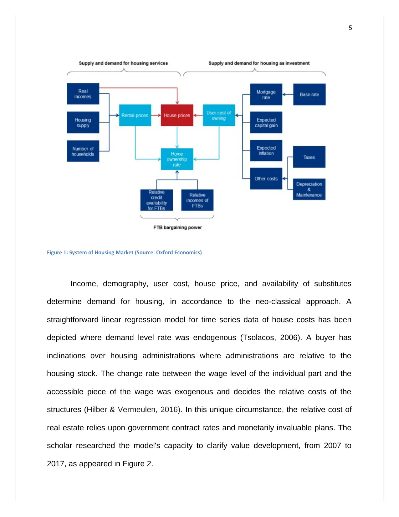
Figure 1: System of Housing Market (Source: Oxford Economics)
Income, demography, user cost, house price, and availability of substitutes
determine demand for housing, in accordance to the neo-classical approach. A
straightforward linear regression model for time series data of house costs has been
depicted where demand level rate was endogenous (Tsolacos, 2006). A buyer has
inclinations over housing administrations where administrations are relative to the
housing stock. The change rate between the wage level of the individual part and the
accessible piece of the wage was exogenous and decides the relative costs of the
structures (Hilber & Vermeulen, 2016). In this unique circumstance, the relative cost of
real estate relies upon government contract rates and monetarily invaluable plans. The
scholar researched the model's capacity to clarify value development, from 2007 to
2017, as appeared in Figure 2.
6
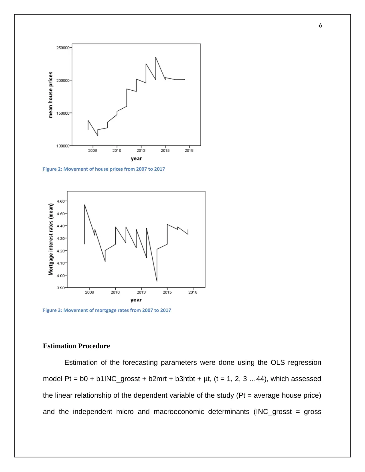
Figure 2: Movement of house prices from 2007 to 2017
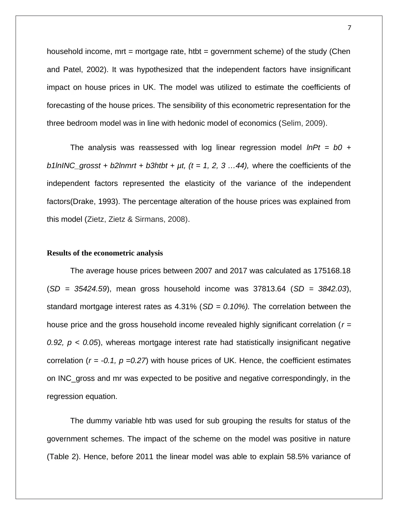
Figure 3: Movement of mortgage rates from 2007 to 2017
Estimation Procedure
Estimation of the forecasting parameters were done using the OLS regression
model Pt = b0 + b1INC_grosst + b2mrt + b3htbt + μt, (t = 1, 2, 3 …44), which assessed
the linear relationship of the dependent variable of the study (Pt = average house price)
and the independent micro and macroeconomic determinants (INC_grosst = gross
Figure 2: Movement of house prices from 2007 to 2017
Figure 3: Movement of mortgage rates from 2007 to 2017
Estimation Procedure
Estimation of the forecasting parameters were done using the OLS regression
model Pt = b0 + b1INC_grosst + b2mrt + b3htbt + μt, (t = 1, 2, 3 …44), which assessed
the linear relationship of the dependent variable of the study (Pt = average house price)
and the independent micro and macroeconomic determinants (INC_grosst = gross
⊘ This is a preview!⊘
Do you want full access?
Subscribe today to unlock all pages.
Trusted by 1+ million students worldwide
7
household income, mrt = mortgage rate, htbt = government scheme) of the study (Chen
and Patel, 2002). It was hypothesized that the independent factors have insignificant
impact on house prices in UK. The model was utilized to estimate the coefficients of
forecasting of the house prices. The sensibility of this econometric representation for the
three bedroom model was in line with hedonic model of economics (Selim, 2009).
The analysis was reassessed with log linear regression model lnPt = b0 +
b1lnINC_grosst + b2lnmrt + b3htbt + μt, (t = 1, 2, 3 …44), where the coefficients of the
independent factors represented the elasticity of the variance of the independent
factors(Drake, 1993). The percentage alteration of the house prices was explained from
this model (Zietz, Zietz & Sirmans, 2008).
Results of the econometric analysis
The average house prices between 2007 and 2017 was calculated as 175168.18
(SD = 35424.59), mean gross household income was 37813.64 (SD = 3842.03),
standard mortgage interest rates as 4.31% (SD = 0.10%). The correlation between the
house price and the gross household income revealed highly significant correlation (r =
0.92, p < 0.05), whereas mortgage interest rate had statistically insignificant negative
correlation (r = -0.1, p =0.27) with house prices of UK. Hence, the coefficient estimates
on INC_gross and mr was expected to be positive and negative correspondingly, in the
regression equation.
The dummy variable htb was used for sub grouping the results for status of the
government schemes. The impact of the scheme on the model was positive in nature
(Table 2). Hence, before 2011 the linear model was able to explain 58.5% variance of
Paraphrase This Document
Need a fresh take? Get an instant paraphrase of this document with our AI Paraphraser
8
house prices and interestingly, the coefficient of mortgage interest rate had positive
effect on the house prices. Post 2011, the government scheme assisted people in
buying homes (Table 3). The model explained mere 41.4% variation of the house
prices, and the impact of gross income increased along with usual negative impact of
mortgage interest rates.
The constant term or the coefficient of the regression term signified the
hypothetical average price of houses in UK in absence of individual income and
mortgage rate. But in reality, for non zero values of the independent variables, there
was no intrinsic meaning for b0. The error term (“μ” term) represents the residuals,
which signifies the difference between the actual and predicted values of house prices.
This additional term removed the possibility of error in the calculated house prices.
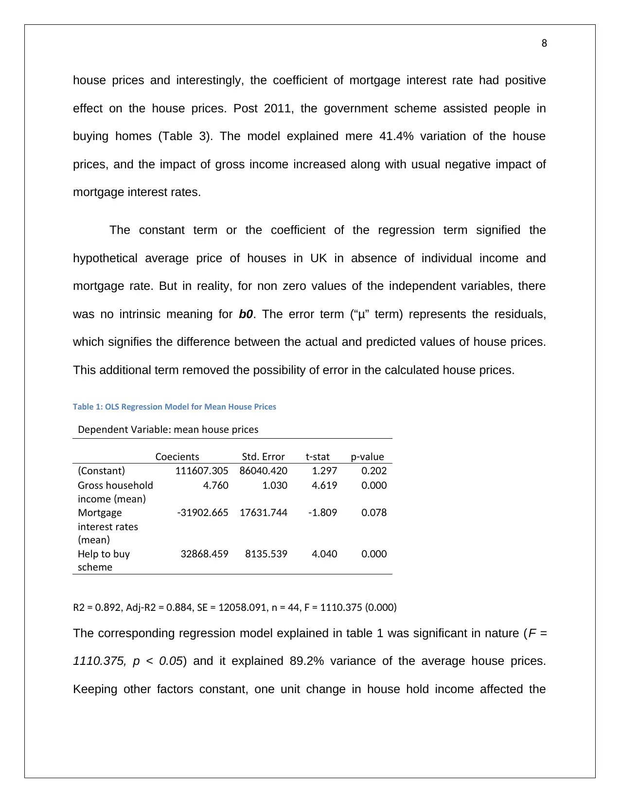
Table 1: OLS Regression Model for Mean House Prices
Dependent Variable mean house prices:
Coefficients Std rror. E t stat- p value-
Constant( ) 111607.305 86040.420 1.297 0.202
ross householdG
income mean( )
4.760 1.030 4.619 0.000
Mortgage
interest rates
mean( )
-31902.665 17631.744 -1.809 0.078
elp to buyH
scheme
32868.459 8135.539 4.040 0.000
R Adj R S n2 = 0.892, - 2 = 0.884, E = 12058.091, = 44, F = 1110.375 (0.000)
The corresponding regression model explained in table 1 was significant in nature (F =
1110.375, p < 0.05) and it explained 89.2% variance of the average house prices.
Keeping other factors constant, one unit change in house hold income affected the
house prices and interestingly, the coefficient of mortgage interest rate had positive
effect on the house prices. Post 2011, the government scheme assisted people in
buying homes (Table 3). The model explained mere 41.4% variation of the house
prices, and the impact of gross income increased along with usual negative impact of
mortgage interest rates.
The constant term or the coefficient of the regression term signified the
hypothetical average price of houses in UK in absence of individual income and
mortgage rate. But in reality, for non zero values of the independent variables, there
was no intrinsic meaning for b0. The error term (“μ” term) represents the residuals,
which signifies the difference between the actual and predicted values of house prices.
This additional term removed the possibility of error in the calculated house prices.
Table 1: OLS Regression Model for Mean House Prices
Dependent Variable mean house prices:
Coefficients Std rror. E t stat- p value-
Constant( ) 111607.305 86040.420 1.297 0.202
ross householdG
income mean( )
4.760 1.030 4.619 0.000
Mortgage
interest rates
mean( )
-31902.665 17631.744 -1.809 0.078
elp to buyH
scheme
32868.459 8135.539 4.040 0.000
R Adj R S n2 = 0.892, - 2 = 0.884, E = 12058.091, = 44, F = 1110.375 (0.000)
The corresponding regression model explained in table 1 was significant in nature (F =
1110.375, p < 0.05) and it explained 89.2% variance of the average house prices.
Keeping other factors constant, one unit change in house hold income affected the
9
house price by 4.76 times. For one percent change in mortgage rate the average house
price was appeared to be negatively affected.
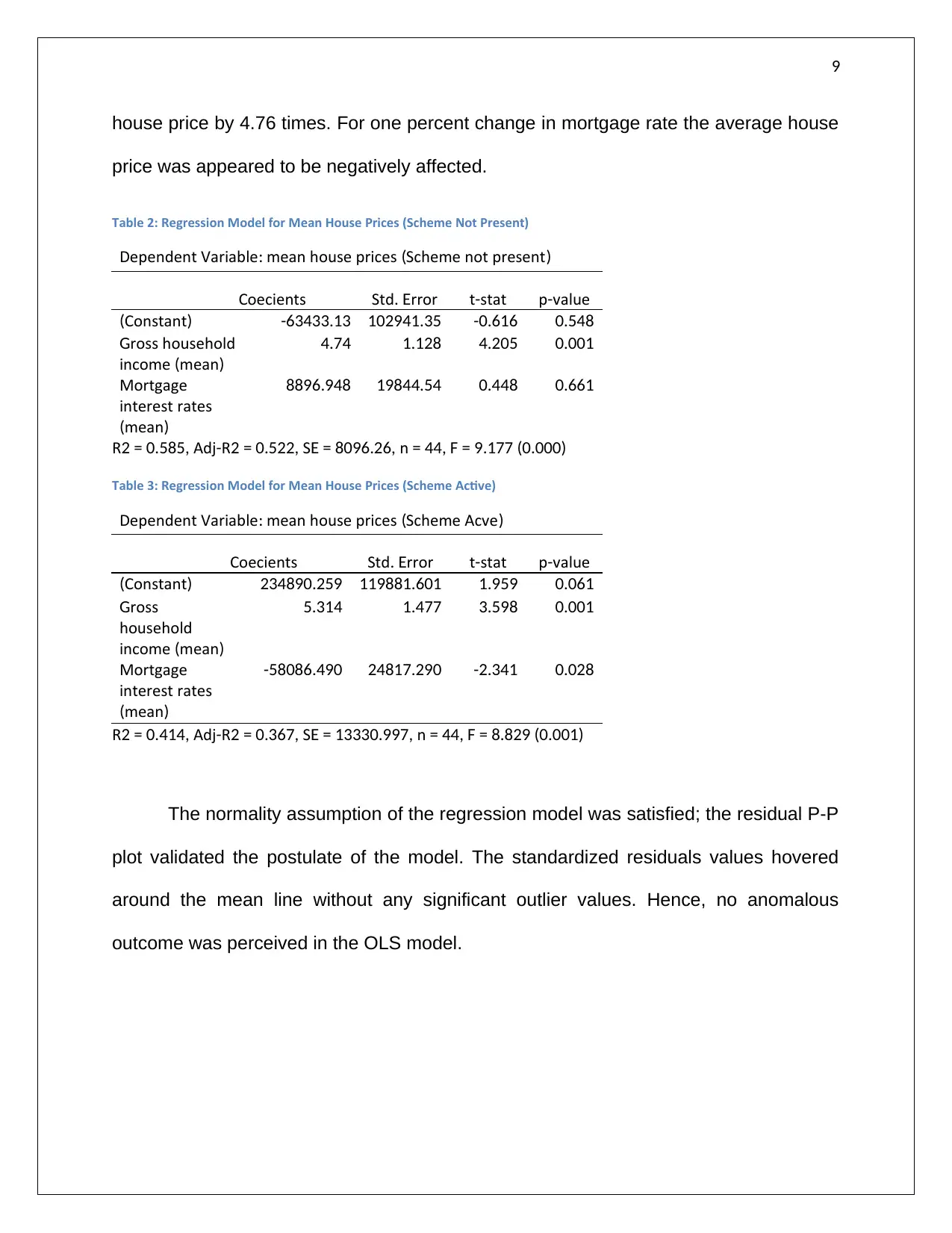
Table 2: Regression Model for Mean House Prices (Scheme Not Present)
Dependent Variable mean house prices Scheme not present: ( )
Coefficients Std rror. E t stat- p value-
Constant( ) -63433.13 102941.35 -0.616 0.548
ross householdG
income mean( )
4.74 1.128 4.205 0.001
Mortgage
interest rates
mean( )
8896.948 19844.54 0.448 0.661
R Adj R S n2 = 0.585, - 2 = 0.522, E = 8096.26, = 44, F = 9.177 (0.000)
Table 3: Regression Model for Mean House Prices (Scheme Active)
Dependent Variable mean house prices Scheme Active: ( )
Coefficients Std rror. E t stat- p value-
Constant( ) 234890.259 119881.601 1.959 0.061
rossG
household
income mean( )
5.314 1.477 3.598 0.001
Mortgage
interest rates
mean( )
-58086.490 24817.290 -2.341 0.028
R Adj R S n2 = 0.414, - 2 = 0.367, E = 13330.997, = 44, F = 8.829 (0.001)
The normality assumption of the regression model was satisfied; the residual P-P
plot validated the postulate of the model. The standardized residuals values hovered
around the mean line without any significant outlier values. Hence, no anomalous
outcome was perceived in the OLS model.
house price by 4.76 times. For one percent change in mortgage rate the average house
price was appeared to be negatively affected.
Table 2: Regression Model for Mean House Prices (Scheme Not Present)
Dependent Variable mean house prices Scheme not present: ( )
Coefficients Std rror. E t stat- p value-
Constant( ) -63433.13 102941.35 -0.616 0.548
ross householdG
income mean( )
4.74 1.128 4.205 0.001
Mortgage
interest rates
mean( )
8896.948 19844.54 0.448 0.661
R Adj R S n2 = 0.585, - 2 = 0.522, E = 8096.26, = 44, F = 9.177 (0.000)
Table 3: Regression Model for Mean House Prices (Scheme Active)
Dependent Variable mean house prices Scheme Active: ( )
Coefficients Std rror. E t stat- p value-
Constant( ) 234890.259 119881.601 1.959 0.061
rossG
household
income mean( )
5.314 1.477 3.598 0.001
Mortgage
interest rates
mean( )
-58086.490 24817.290 -2.341 0.028
R Adj R S n2 = 0.414, - 2 = 0.367, E = 13330.997, = 44, F = 8.829 (0.001)
The normality assumption of the regression model was satisfied; the residual P-P
plot validated the postulate of the model. The standardized residuals values hovered
around the mean line without any significant outlier values. Hence, no anomalous
outcome was perceived in the OLS model.
⊘ This is a preview!⊘
Do you want full access?
Subscribe today to unlock all pages.
Trusted by 1+ million students worldwide
10
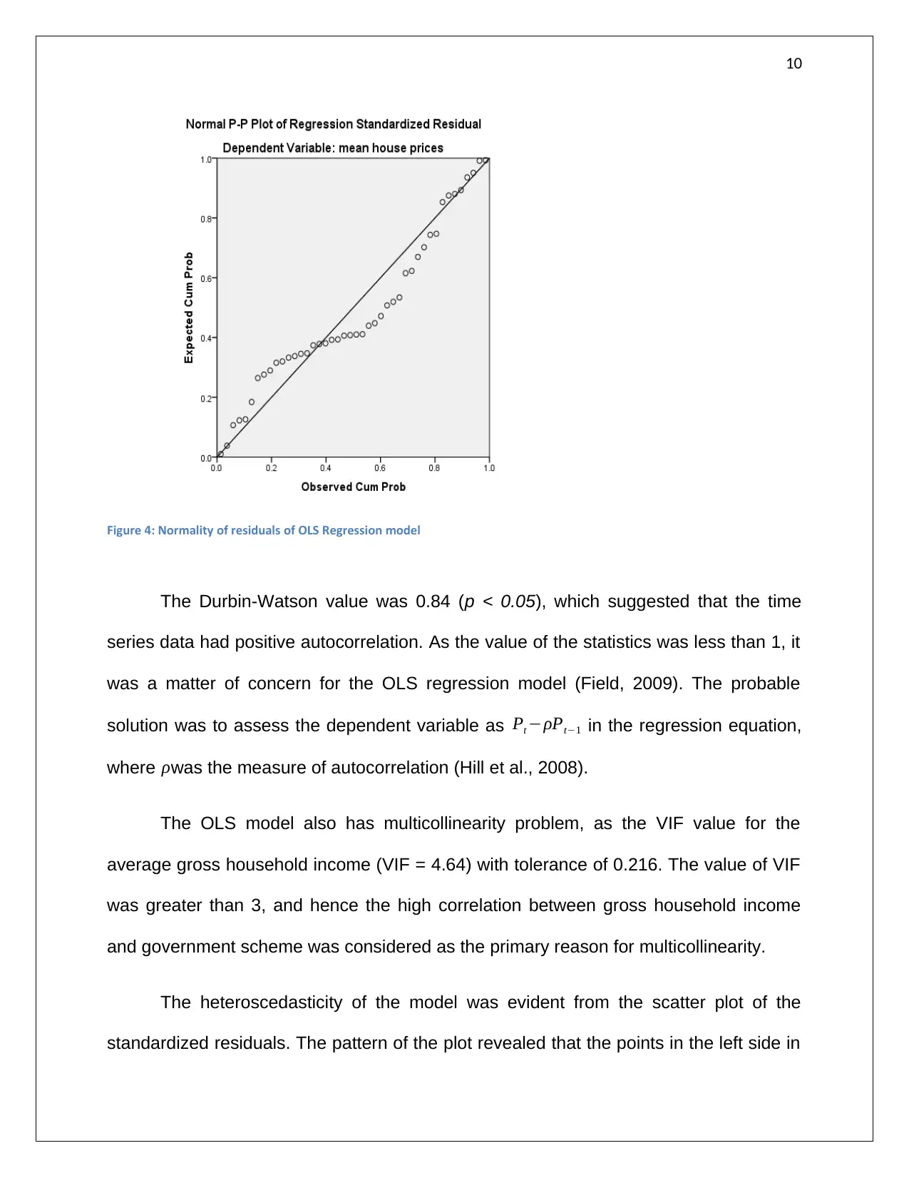
Figure 4: Normality of residuals of OLS Regression model
The Durbin-Watson value was 0.84 (p < 0.05), which suggested that the time
series data had positive autocorrelation. As the value of the statistics was less than 1, it
was a matter of concern for the OLS regression model (Field, 2009). The probable
solution was to assess the dependent variable as Pt −ρPt−1 in the regression equation,
where ρwas the measure of autocorrelation (Hill et al., 2008).
The OLS model also has multicollinearity problem, as the VIF value for the
average gross household income (VIF = 4.64) with tolerance of 0.216. The value of VIF
was greater than 3, and hence the high correlation between gross household income
and government scheme was considered as the primary reason for multicollinearity.
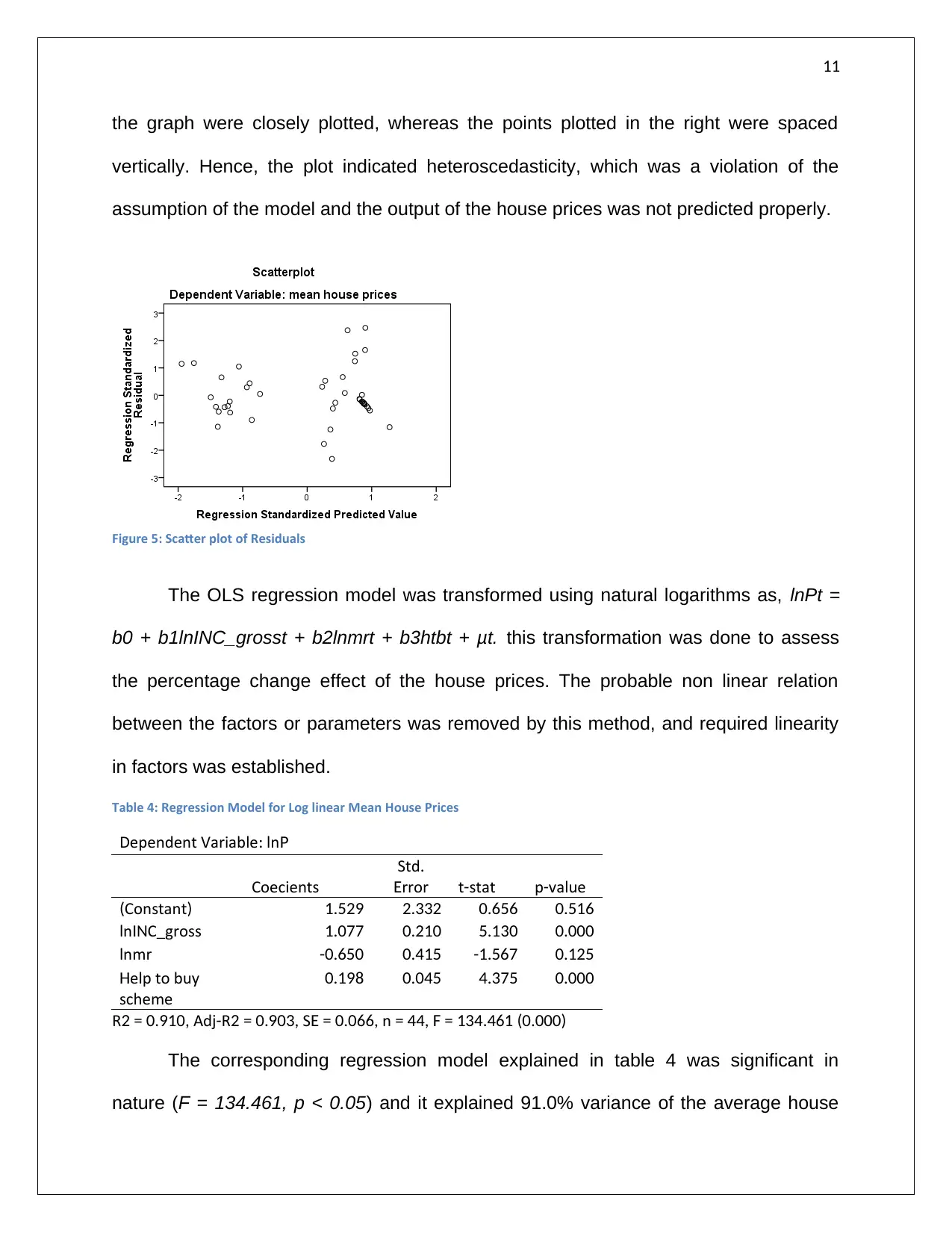
The heteroscedasticity of the model was evident from the scatter plot of the
standardized residuals. The pattern of the plot revealed that the points in the left side in
Figure 4: Normality of residuals of OLS Regression model
The Durbin-Watson value was 0.84 (p < 0.05), which suggested that the time
series data had positive autocorrelation. As the value of the statistics was less than 1, it
was a matter of concern for the OLS regression model (Field, 2009). The probable
solution was to assess the dependent variable as Pt −ρPt−1 in the regression equation,
where ρwas the measure of autocorrelation (Hill et al., 2008).
The OLS model also has multicollinearity problem, as the VIF value for the
average gross household income (VIF = 4.64) with tolerance of 0.216. The value of VIF
was greater than 3, and hence the high correlation between gross household income
and government scheme was considered as the primary reason for multicollinearity.
The heteroscedasticity of the model was evident from the scatter plot of the
standardized residuals. The pattern of the plot revealed that the points in the left side in
Paraphrase This Document
Need a fresh take? Get an instant paraphrase of this document with our AI Paraphraser
11
the graph were closely plotted, whereas the points plotted in the right were spaced
vertically. Hence, the plot indicated heteroscedasticity, which was a violation of the
assumption of the model and the output of the house prices was not predicted properly.
Figure 5: Scatter plot of Residuals
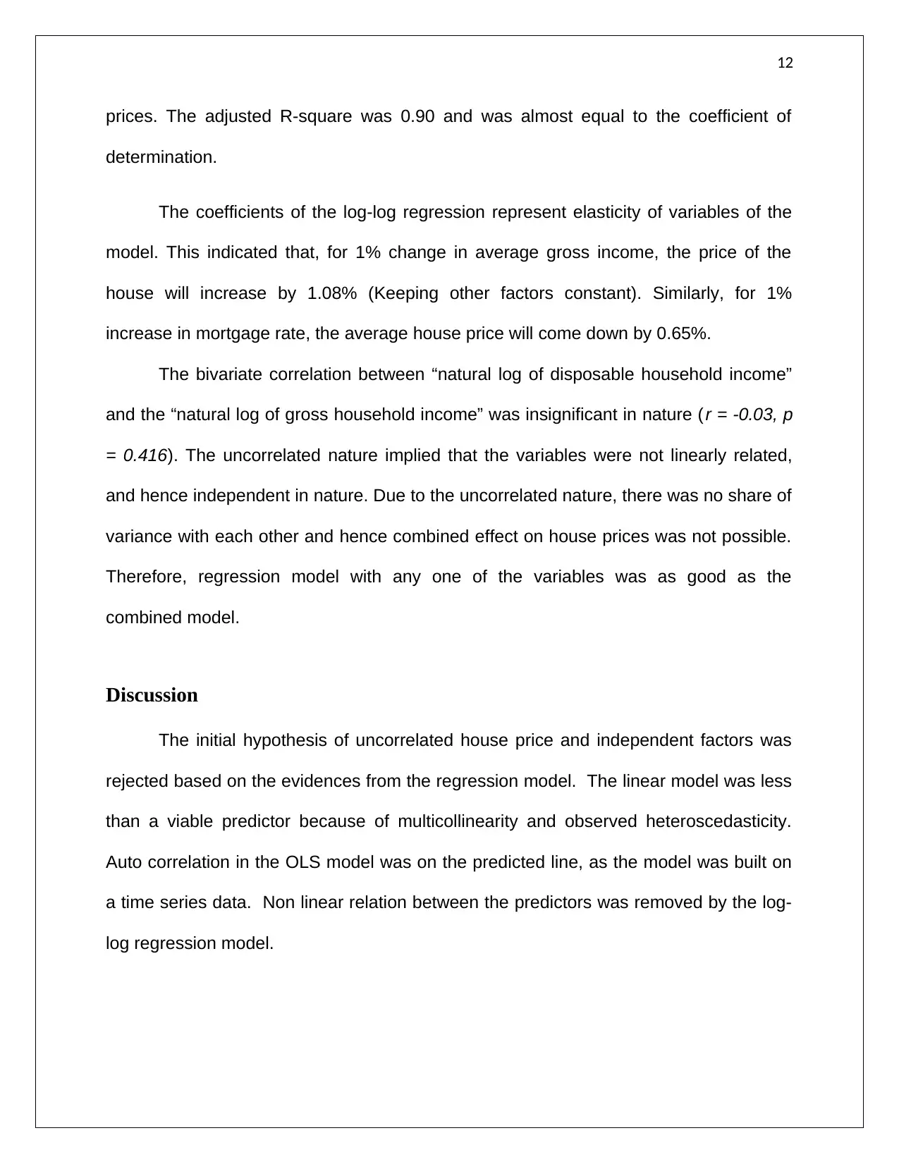
The OLS regression model was transformed using natural logarithms as, lnPt =
b0 + b1lnINC_grosst + b2lnmrt + b3htbt + μt. this transformation was done to assess
the percentage change effect of the house prices. The probable non linear relation
between the factors or parameters was removed by this method, and required linearity
in factors was established.
Table 4: Regression Model for Log linear Mean House Prices
Dependent Variable ln: P
Coefficients
Std.
rrorE t stat- p value-
Constant( ) 1.529 2.332 0.656 0.516
ln C grossIN _ 1.077 0.210 5.130 0.000
lnmr -0.650 0.415 -1.567 0.125
elp to buyH
scheme
0.198 0.045 4.375 0.000
R Adj R S n2 = 0.910, - 2 = 0.903, E = 0.066, = 44, F = 134.461 (0.000)
The corresponding regression model explained in table 4 was significant in
nature (F = 134.461, p < 0.05) and it explained 91.0% variance of the average house
the graph were closely plotted, whereas the points plotted in the right were spaced
vertically. Hence, the plot indicated heteroscedasticity, which was a violation of the
assumption of the model and the output of the house prices was not predicted properly.
Figure 5: Scatter plot of Residuals
The OLS regression model was transformed using natural logarithms as, lnPt =
b0 + b1lnINC_grosst + b2lnmrt + b3htbt + μt. this transformation was done to assess
the percentage change effect of the house prices. The probable non linear relation
between the factors or parameters was removed by this method, and required linearity
in factors was established.
Table 4: Regression Model for Log linear Mean House Prices
Dependent Variable ln: P
Coefficients
Std.
rrorE t stat- p value-
Constant( ) 1.529 2.332 0.656 0.516
ln C grossIN _ 1.077 0.210 5.130 0.000
lnmr -0.650 0.415 -1.567 0.125
elp to buyH
scheme
0.198 0.045 4.375 0.000
R Adj R S n2 = 0.910, - 2 = 0.903, E = 0.066, = 44, F = 134.461 (0.000)
The corresponding regression model explained in table 4 was significant in
nature (F = 134.461, p < 0.05) and it explained 91.0% variance of the average house
12
prices. The adjusted R-square was 0.90 and was almost equal to the coefficient of
determination.
The coefficients of the log-log regression represent elasticity of variables of the
model. This indicated that, for 1% change in average gross income, the price of the
house will increase by 1.08% (Keeping other factors constant). Similarly, for 1%
increase in mortgage rate, the average house price will come down by 0.65%.
The bivariate correlation between “natural log of disposable household income”
and the “natural log of gross household income” was insignificant in nature ( r = -0.03, p
= 0.416). The uncorrelated nature implied that the variables were not linearly related,
and hence independent in nature. Due to the uncorrelated nature, there was no share of
variance with each other and hence combined effect on house prices was not possible.
Therefore, regression model with any one of the variables was as good as the
combined model.
Discussion
The initial hypothesis of uncorrelated house price and independent factors was
rejected based on the evidences from the regression model. The linear model was less
than a viable predictor because of multicollinearity and observed heteroscedasticity.
Auto correlation in the OLS model was on the predicted line, as the model was built on
a time series data. Non linear relation between the predictors was removed by the log-
log regression model.
⊘ This is a preview!⊘
Do you want full access?
Subscribe today to unlock all pages.
Trusted by 1+ million students worldwide
1 out of 24
Related Documents


Your All-in-One AI-Powered Toolkit for Academic Success.
+13062052269
info@desklib.com
Available 24*7 on WhatsApp / Email
![[object Object]](/_next/static/media/star-bottom.7253800d.svg)
Unlock your academic potential
Copyright © 2020–2026 A2Z Services. All Rights Reserved. Developed and managed by ZUCOL.