BUSSSBF Course Assignment: Statistical Analysis of Household Data

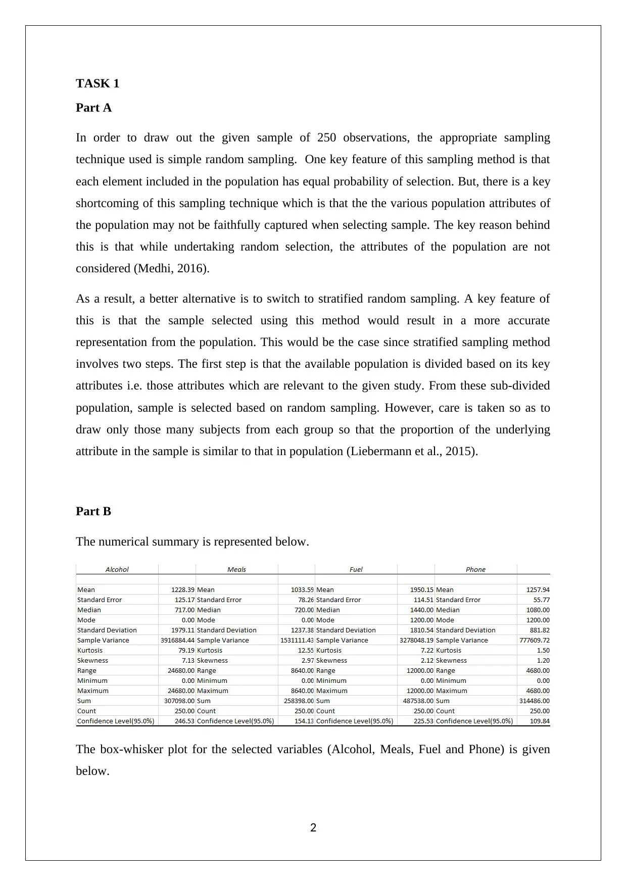
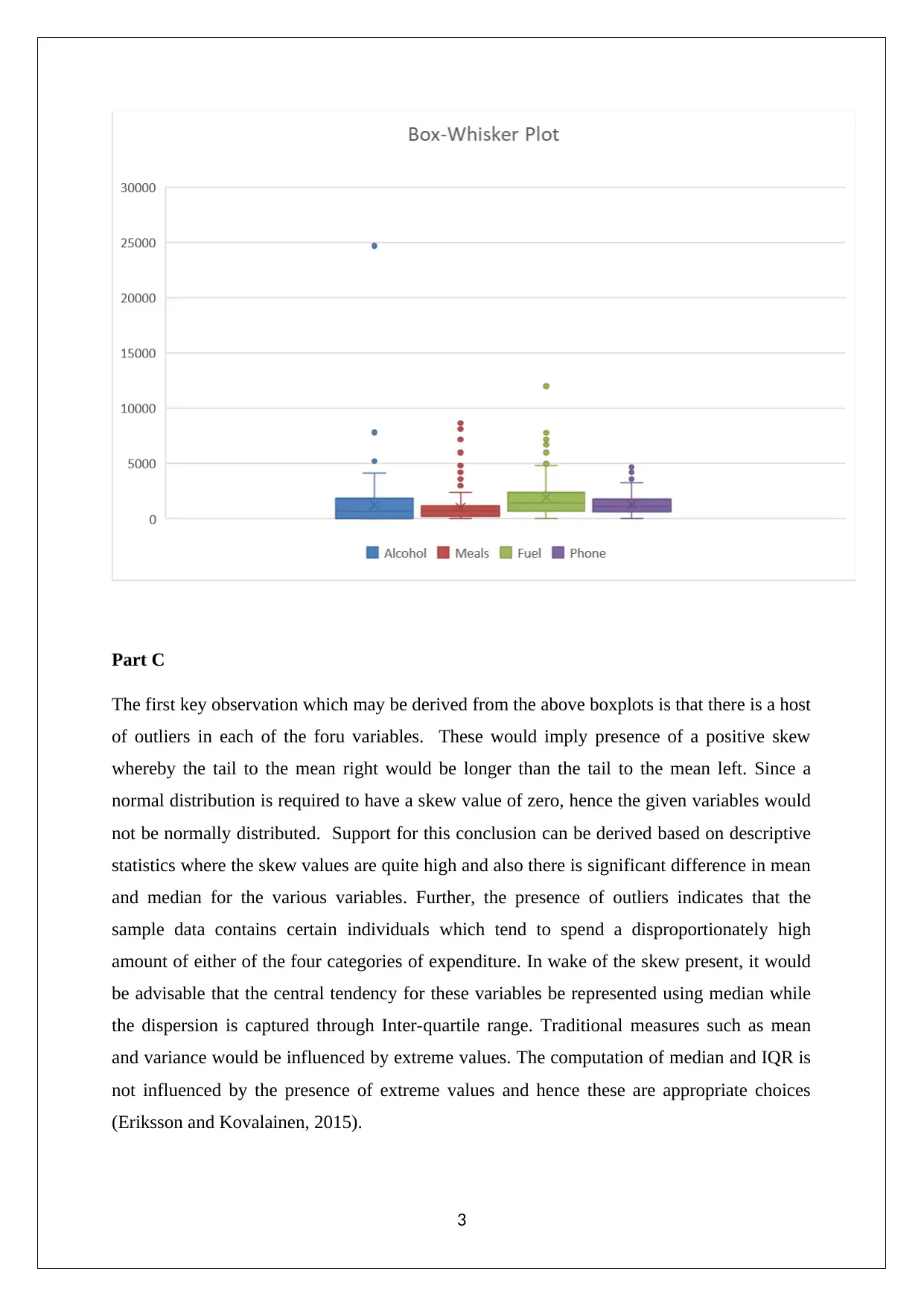
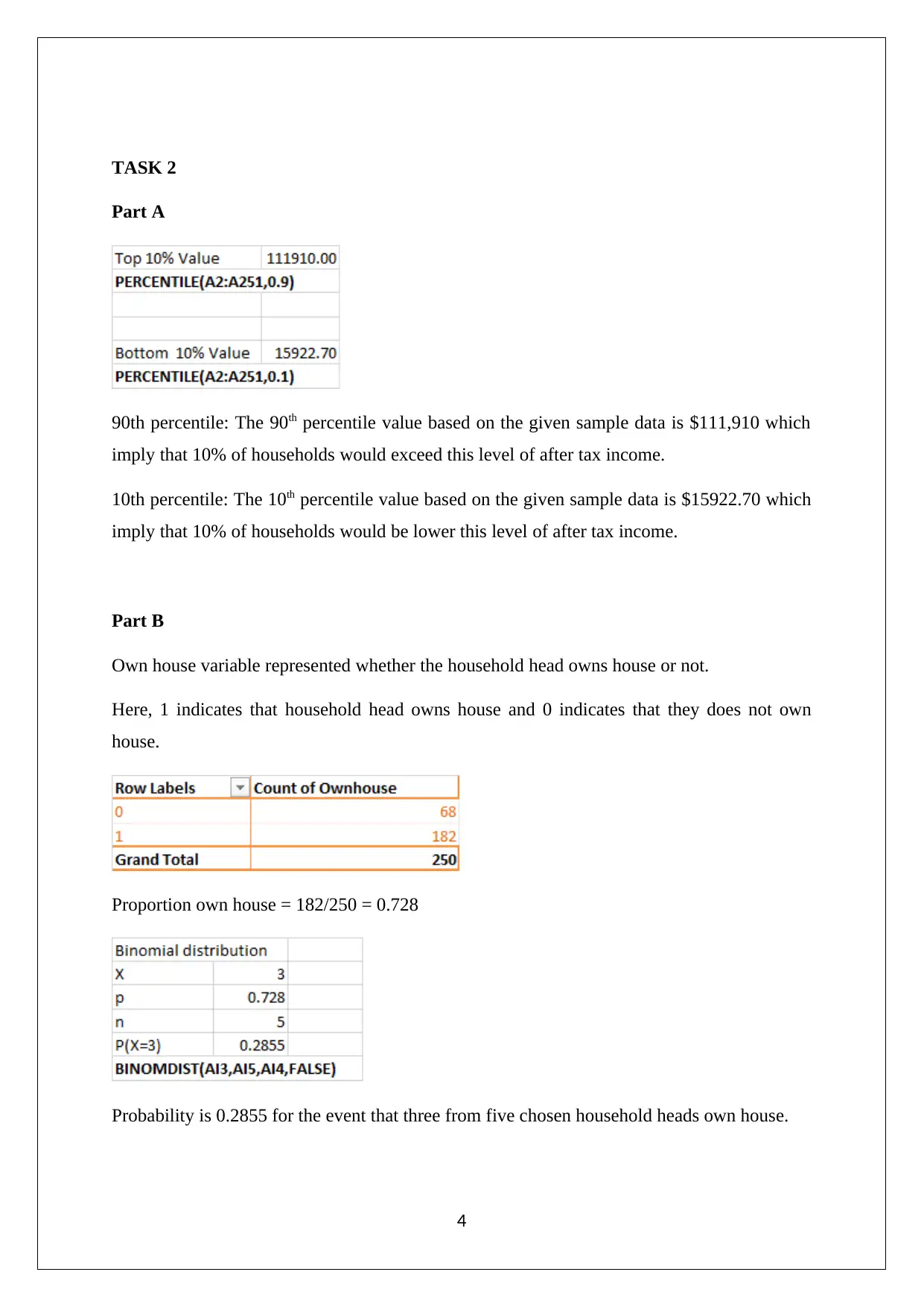
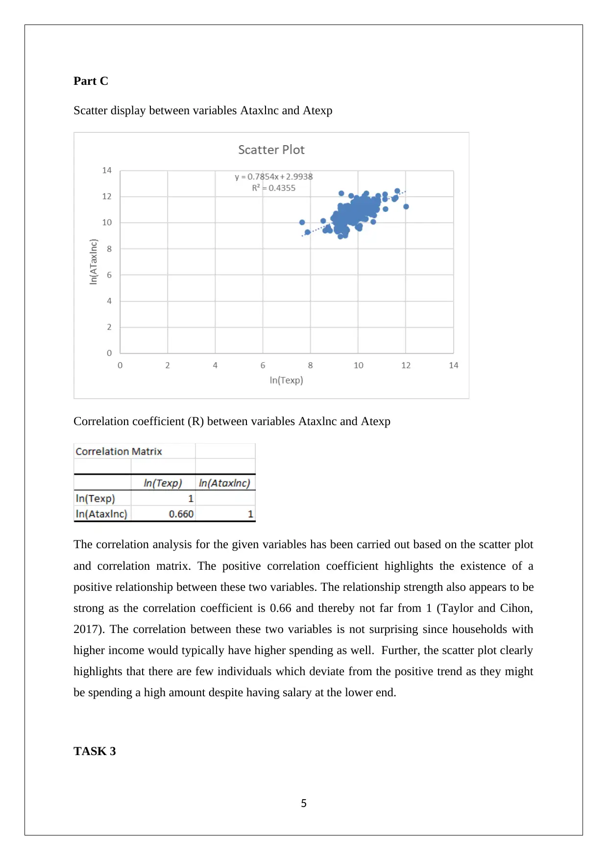
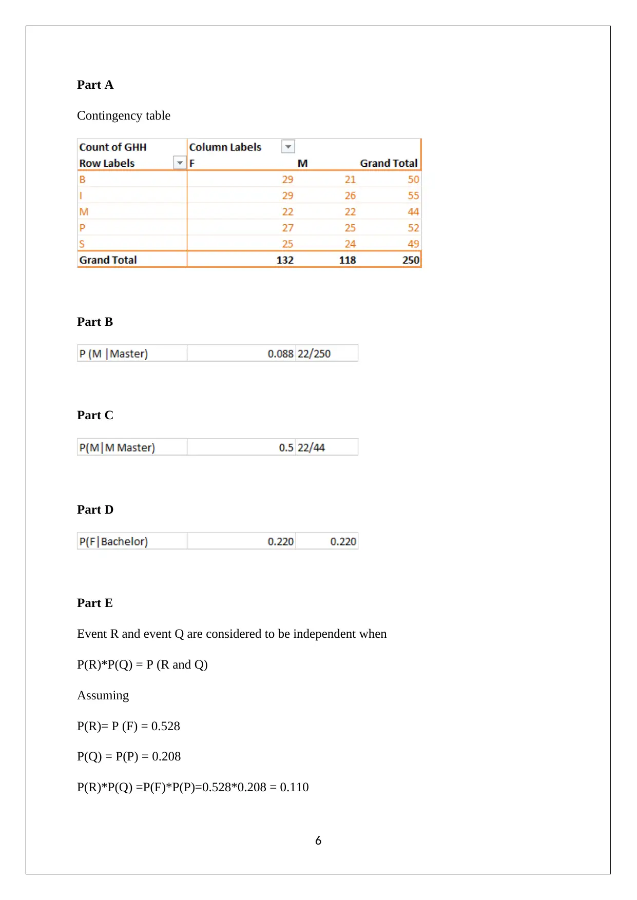
This assignment analyzes household data using statistical methods, addressing tasks related to sampling techniques, descriptive statistics, and probability. The student begins by employing simple random sampling to extract a sample of 250 observations and justifies the choice of this sampling method. Descriptive statistics are then calculated and visualized using box-whisker plots for variables such as alcohol, meals, fuel, and phone expenditure. The presence of outliers and the non-normality of the data distribution are discussed, along with the appropriate measures of central tendency and dispersion. Further, the assignment explores the 90th and 10th percentiles of after-tax income, the probability of household characteristics, and the correlation between variables using scatter plots and correlation coefficients. Finally, the assignment constructs a contingency table and calculates probabilities based on gender and education level, evaluating the independence of events.

STATISTICS FOR BUSINESS AND FINANCE
STUDENT ID:
[Pick the date]

TASK 1
Part A
In order to draw out the given sample of 250 observations, the appropriate sampling
technique used is simple random sampling. One key feature of this sampling method is that
each element included in the population has equal probability of selection. But, there is a key
shortcoming of this sampling technique which is that the the various population attributes of
the population may not be faithfully captured when selecting sample. The key reason behind
this is that while undertaking random selection, the attributes of the population are not
considered (Medhi, 2016).
As a result, a better alternative is to switch to stratified random sampling. A key feature of
this is that the sample selected using this method would result in a more accurate
representation from the population. This would be the case since stratified sampling method
involves two steps. The first step is that the available population is divided based on its key
attributes i.e. those attributes which are relevant to the given study. From these sub-divided
population, sample is selected based on random sampling. However, care is taken so as to
draw only those many subjects from each group so that the proportion of the underlying
attribute in the sample is similar to that in population (Liebermann et al., 2015).
Part B
The numerical summary is represented below.
The box-whisker plot for the selected variables (Alcohol, Meals, Fuel and Phone) is given
below.
2

Part C
The first key observation which may be derived from the above boxplots is that there is a host
of outliers in each of the foru variables. These would imply presence of a positive skew
whereby the tail to the mean right would be longer than the tail to the mean left. Since a
normal distribution is required to have a skew value of zero, hence the given variables would
not be normally distributed. Support for this conclusion can be derived based on descriptive
statistics where the skew values are quite high and also there is significant difference in mean
and median for the various variables. Further, the presence of outliers indicates that the
sample data contains certain individuals which tend to spend a disproportionately high
amount of either of the four categories of expenditure. In wake of the skew present, it would
be advisable that the central tendency for these variables be represented using median while
the dispersion is captured through Inter-quartile range. Traditional measures such as mean
and variance would be influenced by extreme values. The computation of median and IQR is
not influenced by the presence of extreme values and hence these are appropriate choices
(Eriksson and Kovalainen, 2015).
3

TASK 2
Part A
90th percentile: The 90th percentile value based on the given sample data is $111,910 which
imply that 10% of households would exceed this level of after tax income.
10th percentile: The 10th percentile value based on the given sample data is $15922.70 which
imply that 10% of households would be lower this level of after tax income.
Part B
Own house variable represented whether the household head owns house or not.
Here, 1 indicates that household head owns house and 0 indicates that they does not own
house.
Proportion own house = 182/250 = 0.728
Probability is 0.2855 for the event that three from five chosen household heads own house.
4

Part C
Scatter display between variables Ataxlnc and Atexp
Correlation coefficient (R) between variables Ataxlnc and Atexp
The correlation analysis for the given variables has been carried out based on the scatter plot
and correlation matrix. The positive correlation coefficient highlights the existence of a
positive relationship between these two variables. The relationship strength also appears to be
strong as the correlation coefficient is 0.66 and thereby not far from 1 (Taylor and Cihon,
2017). The correlation between these two variables is not surprising since households with
higher income would typically have higher spending as well. Further, the scatter plot clearly
highlights that there are few individuals which deviate from the positive trend as they might
be spending a high amount despite having salary at the lower end.
TASK 3
5

Part A
Contingency table
Part B
Part C
Part D
Part E
Event R and event Q are considered to be independent when
P(R)*P(Q) = P (R and Q)
Assuming
P(R)= P (F) = 0.528
P(Q) = P(P) = 0.208
P(R)*P(Q) =P(F)*P(P)=0.528*0.208 = 0.110
6

P (R and Q) =P (F and P) = 0.108
Clearly, P(R)*P(Q) = P (R and Q) is not equal and thus, it is not independent.
The conclusion can be made that female and being educated by primary education is not
considered as independent events.
7

References
Eriksson, P. and Kovalainen, A. (2015) Quantitative methods in business research. 3rd ed.
London: Sage Publications.
Lieberman, F. J., Nag, B., Hiller, F.S. and Basu, P. (2015) Introduction To Operations
Research. 5th ed.New Delhi: Tata McGraw Hill Publishers.
Medhi, J. (2016) Statistical Methods: An Introductory Text. 4th ed. Sydney: New Age
International.
Taylor, K. J. and Cihon, C. (2017) Statistical Techniques for Data Analysis. 2nd ed.
Melbourne: CRC Press.
8