Household Data Analysis: A Statistical Exploration

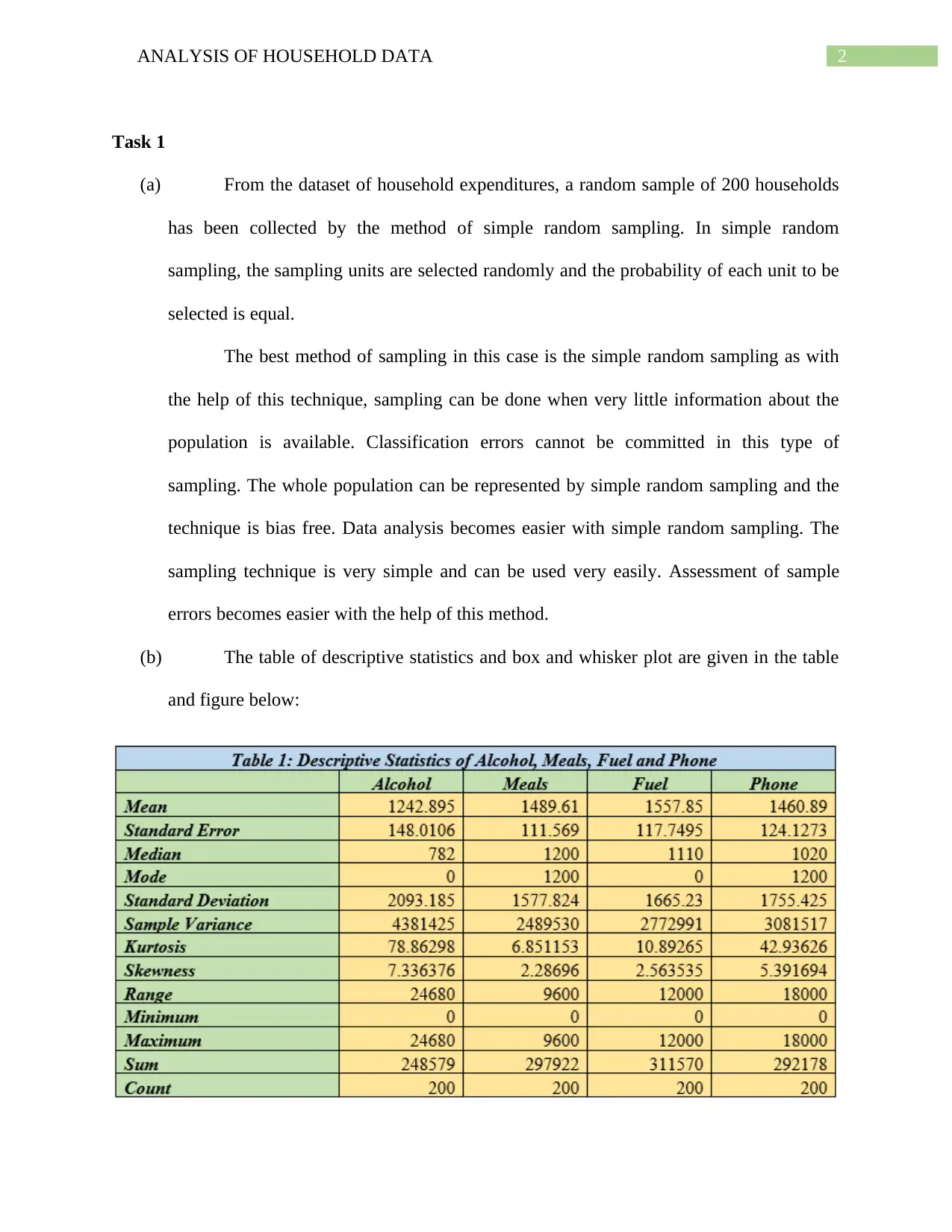
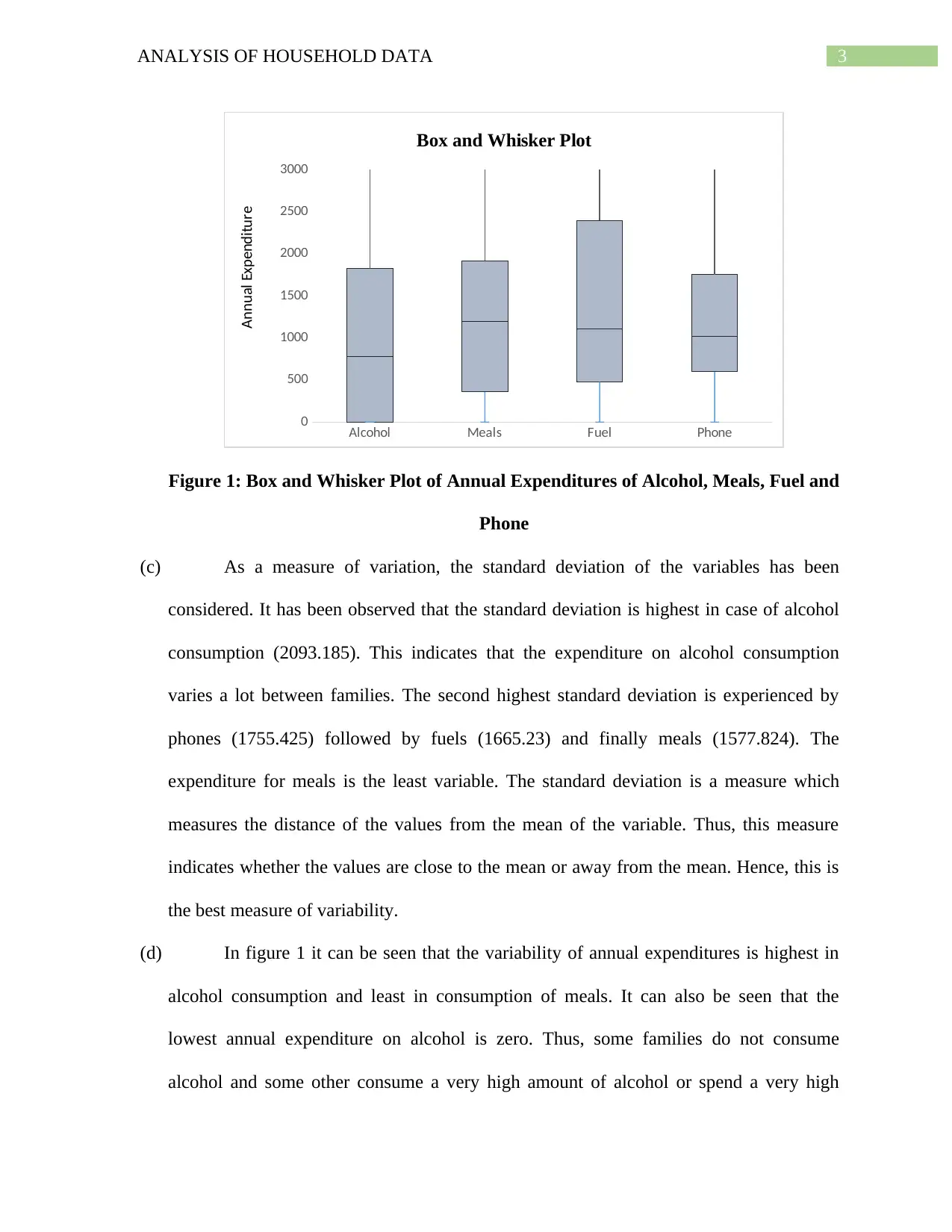
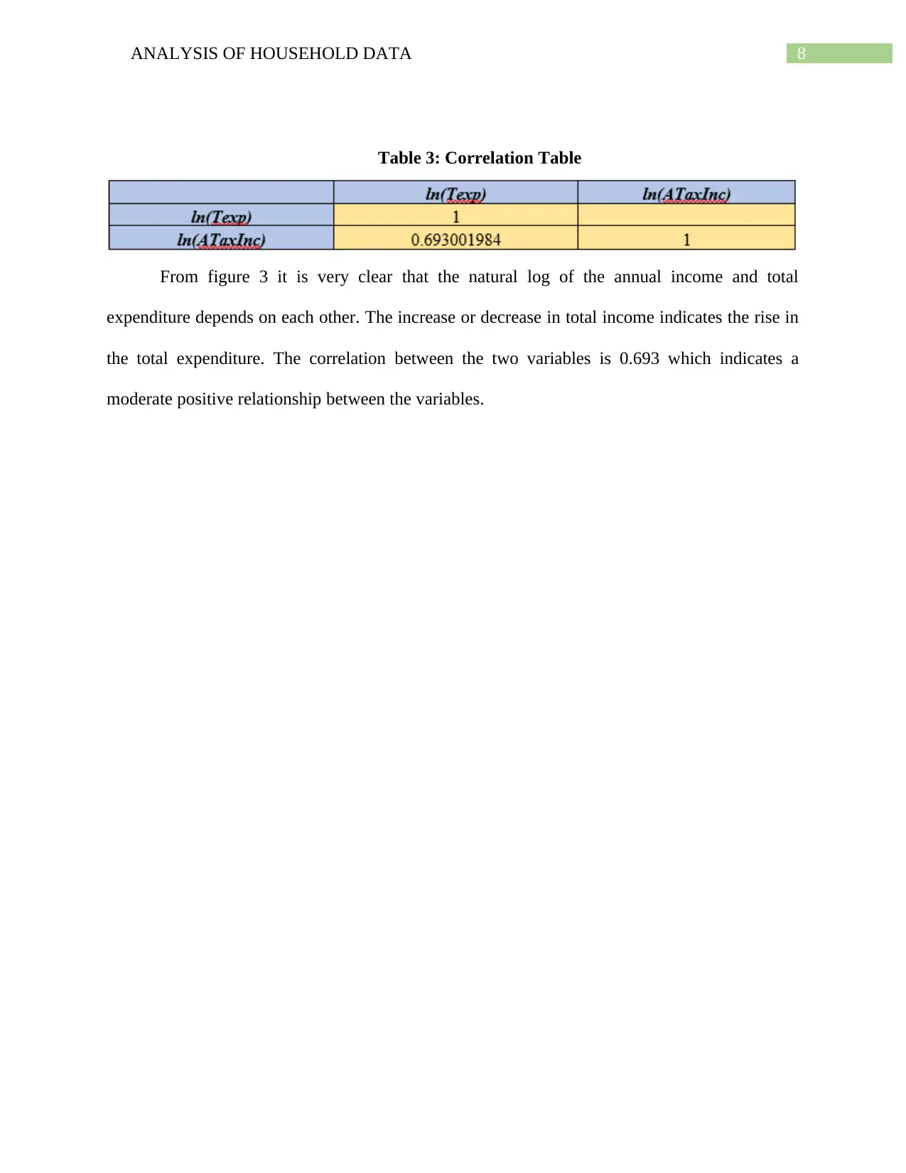
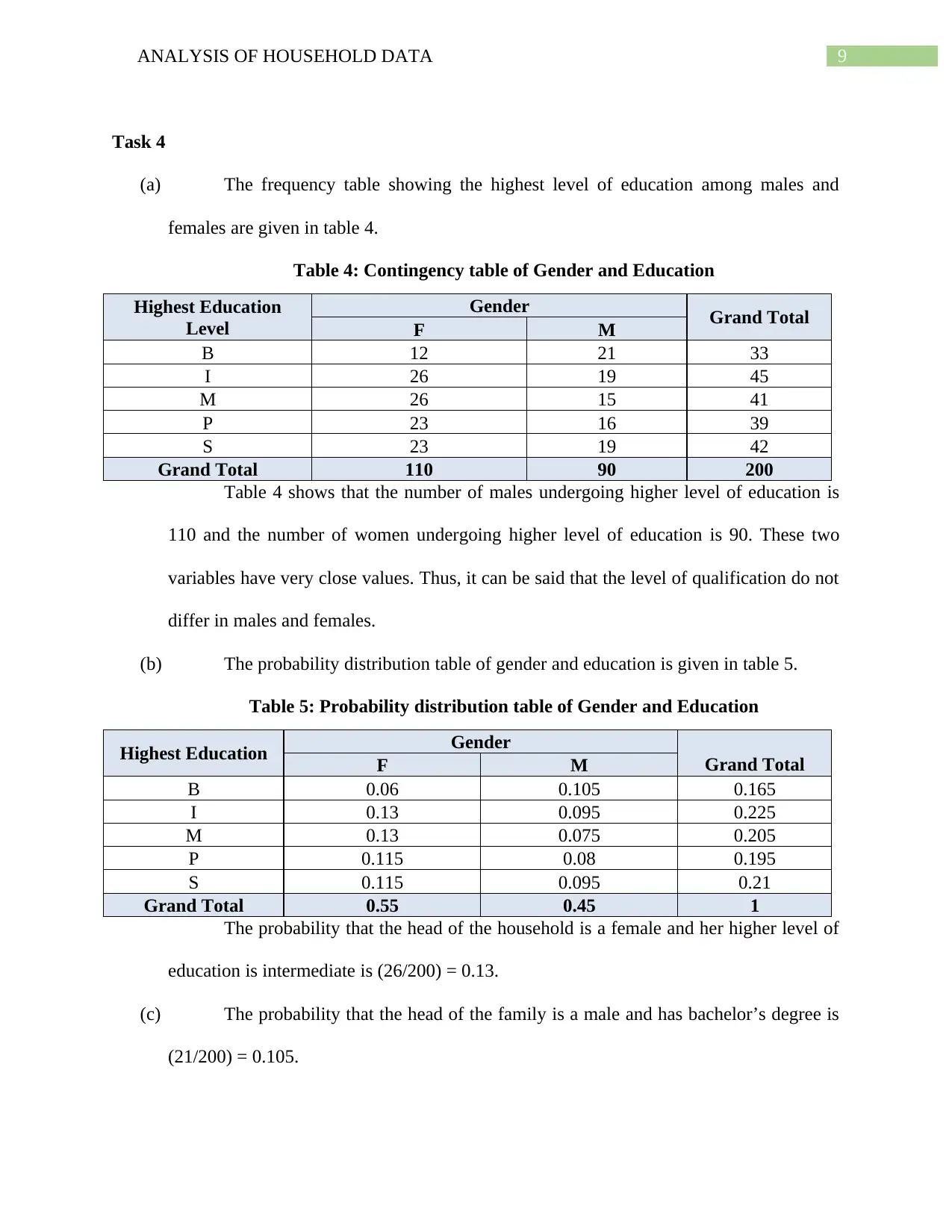
This assignment provides a comprehensive analysis of household data, employing various statistical techniques. It begins with a simple random sample of 200 households, justifying the use of this method for its bias-free nature and ease of data analysis. Descriptive statistics are presented, including a box and whisker plot visualizing annual expenditures on alcohol, meals, fuel, and phone services, with standard deviation used to measure variability. The analysis extends to frequency distribution of utility expenditures, calculating percentages within specified ranges and illustrating the distribution via a histogram. Percentile calculations for after-tax income are performed, alongside probability analysis related to household size and homeownership. A scatterplot examines the relationship between after-tax income and total expenditure, quantified by correlation. Finally, a contingency table explores the relationship between gender and education level within the households, calculating relevant probabilities and testing for independence between variables.

Running Head: ANALYSIS OF HOUSEHOLD DATA
Analysis of Household Data
Name of the Student
Name of the University
Author Note

1ANALYSIS OF HOUSEHOLD DATA
Table of Contents
Task 1...............................................................................................................................................2
Task 2...............................................................................................................................................5
Task 3...............................................................................................................................................7
Task 4...............................................................................................................................................9

2ANALYSIS OF HOUSEHOLD DATA
Task 1
(a) From the dataset of household expenditures, a random sample of 200 households
has been collected by the method of simple random sampling. In simple random
sampling, the sampling units are selected randomly and the probability of each unit to be
selected is equal.
The best method of sampling in this case is the simple random sampling as with
the help of this technique, sampling can be done when very little information about the
population is available. Classification errors cannot be committed in this type of
sampling. The whole population can be represented by simple random sampling and the
technique is bias free. Data analysis becomes easier with simple random sampling. The
sampling technique is very simple and can be used very easily. Assessment of sample
errors becomes easier with the help of this method.
(b) The table of descriptive statistics and box and whisker plot are given in the table
and figure below:

3ANALYSIS OF HOUSEHOLD DATA
Alcohol Meals Fuel Phone
0
500
1000
1500
2000
2500
3000
Box and Whisker Plot
Annual Expenditure
Figure 1: Box and Whisker Plot of Annual Expenditures of Alcohol, Meals, Fuel and
Phone
(c) As a measure of variation, the standard deviation of the variables has been
considered. It has been observed that the standard deviation is highest in case of alcohol
consumption (2093.185). This indicates that the expenditure on alcohol consumption
varies a lot between families. The second highest standard deviation is experienced by
phones (1755.425) followed by fuels (1665.23) and finally meals (1577.824). The
expenditure for meals is the least variable. The standard deviation is a measure which
measures the distance of the values from the mean of the variable. Thus, this measure
indicates whether the values are close to the mean or away from the mean. Hence, this is
the best measure of variability.
(d) In figure 1 it can be seen that the variability of annual expenditures is highest in
alcohol consumption and least in consumption of meals. It can also be seen that the
lowest annual expenditure on alcohol is zero. Thus, some families do not consume
alcohol and some other consume a very high amount of alcohol or spend a very high

4ANALYSIS OF HOUSEHOLD DATA
amount on alcohol. On the other hand, every family spends more or less the same amount
on daily meals as this is a necessity. Thus, this explains the least variability in the annual
expenditure for meals. The distribution of the expenditures has a higher mean, followed
by the median and the mode. This indicates that the expenses are higher than the mean
expenses for the families on the consumption of alcohol, fuels, phone and meals.

5ANALYSIS OF HOUSEHOLD DATA
Task 2
(a) The frequency distribution table for the annual expenditure on utilities are given
in the following table:
(b) The required percentages are given as below:
 The percentage of households spending a maximum of $1200 per annum
is 68%.
 The percentage of households having expenditure on utilities between
$1200 and $2400 per annum is (17.5 + 6.5 + 4)% = 28%.
 The percentage of households spending ore than $2400 per annum is (1.5
+ 1 + 1.5) % = 4%.
(c) The histogram showing the expenses on utilities by a household is given in figure
2.

6ANALYSIS OF HOUSEHOLD DATA
0-400 400-800 800-
1200 1200-
1600 1600-
2000 2000-
2400 2400-
2800 2800-
3200 More
than
3200
0
10
20
30
40
50
60
70
Histogram of Utilities
Expenditure on Utilities
Frequencies
Figure 2: Household Expenditure on Utilities
(d) The annual family expenditures are not distributed normally. It can also be seen
that most of the household expenses lies below the average expenditure. Thus, the
expensive goods can only be purchased by a very little proportion of people. On the other
hand, the cheaper utility goods can be afforded by most of the households and thus it
explains the trend in the data.

7ANALYSIS OF HOUSEHOLD DATA
Task 3
(a) The 90th percentile and the 10th percentile are respectively the top and the bottom
90% and 10% of the values of a distribution. In this problem, the annual after tax income
has been considered as the variable. The top 10% annual after tax income is above
$122673.5 and the bottom 10% annual after tax income is below $19842.
(b) The variable OwnHouse indicates whether an individual owns a house or not.
Owning a house is indicated by 1 and 0 otherwise. The mean of the variable OwnHouse
is found to be 0.67 which is more than the half of the values, 0.5. Thus, it can be said that
most of the households own their house.
(c) In the sample of 200 households, the number of households having a family size
of 5 is 17. Thus, the probability that a randomly selected household will have a family
size equal to 5 is given by (17/200) = 0.085.
(d) The scatterplot showing the logarithm values of after tax income and total
expenditure is given in figure 3.
8.500 9.000 9.500 10.000 10.500 11.000 11.500 12.000 12.500 13.000 13.500
0.000
2.000
4.000
6.000
8.000
10.000
12.000
14.000
Scatterplot of ln(ATanInc) vs. ln(Texp)
ln(ATaxInc)
ln(Texp)
Figure 3: Scatterplot of annual after tax income and total expenditure.

8ANALYSIS OF HOUSEHOLD DATA
Table 3: Correlation Table
From figure 3 it is very clear that the natural log of the annual income and total
expenditure depends on each other. The increase or decrease in total income indicates the rise in
the total expenditure. The correlation between the two variables is 0.693 which indicates a
moderate positive relationship between the variables.

9ANALYSIS OF HOUSEHOLD DATA
Task 4
(a) The frequency table showing the highest level of education among males and
females are given in table 4.
Table 4: Contingency table of Gender and Education
Highest Education
Level
Gender Grand Total
F M
B 12 21 33
I 26 19 45
M 26 15 41
P 23 16 39
S 23 19 42
Grand Total 110 90 200
Table 4 shows that the number of males undergoing higher level of education is
110 and the number of women undergoing higher level of education is 90. These two
variables have very close values. Thus, it can be said that the level of qualification do not
differ in males and females.
(b) The probability distribution table of gender and education is given in table 5.
Table 5: Probability distribution table of Gender and Education
Highest Education Gender
Grand TotalF M
B 0.06 0.105 0.165
I 0.13 0.095 0.225
M 0.13 0.075 0.205
P 0.115 0.08 0.195
S 0.115 0.095 0.21
Grand Total 0.55 0.45 1
The probability that the head of the household is a female and her higher level of
education is intermediate is (26/200) = 0.13.
(c) The probability that the head of the family is a male and has bachelor’s degree is
(21/200) = 0.105.

10ANALYSIS OF HOUSEHOLD DATA
(d) The proportion of having secondary as the highest degree from among females is
((23+23)/200) = 0.23.
(e) Two events are said to be independent if the product of the probabilities of the
two events separately are equal to the probability of the occurrence of the two events
together. Thus,
The probability of gender of a household head being male is (90/200) = 0.45.
The probability of having a master’s degree is (41/200) = 0.205.
The probability of a household head being male and having a master’s degree is (15/200)
= 0.075.
Now, (0.45*0.205) = 0.092 which is not equal to 0.075.
Thus, the two events are dependent.