STAT6003: Statistical Analysis of Sydney Housing Market Case Study

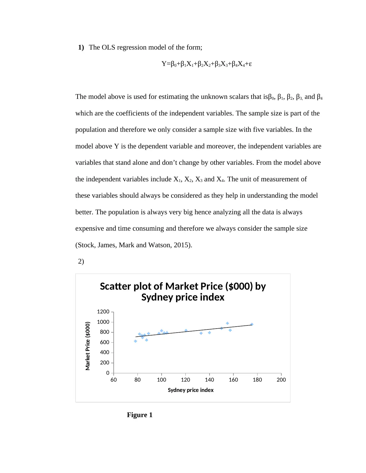
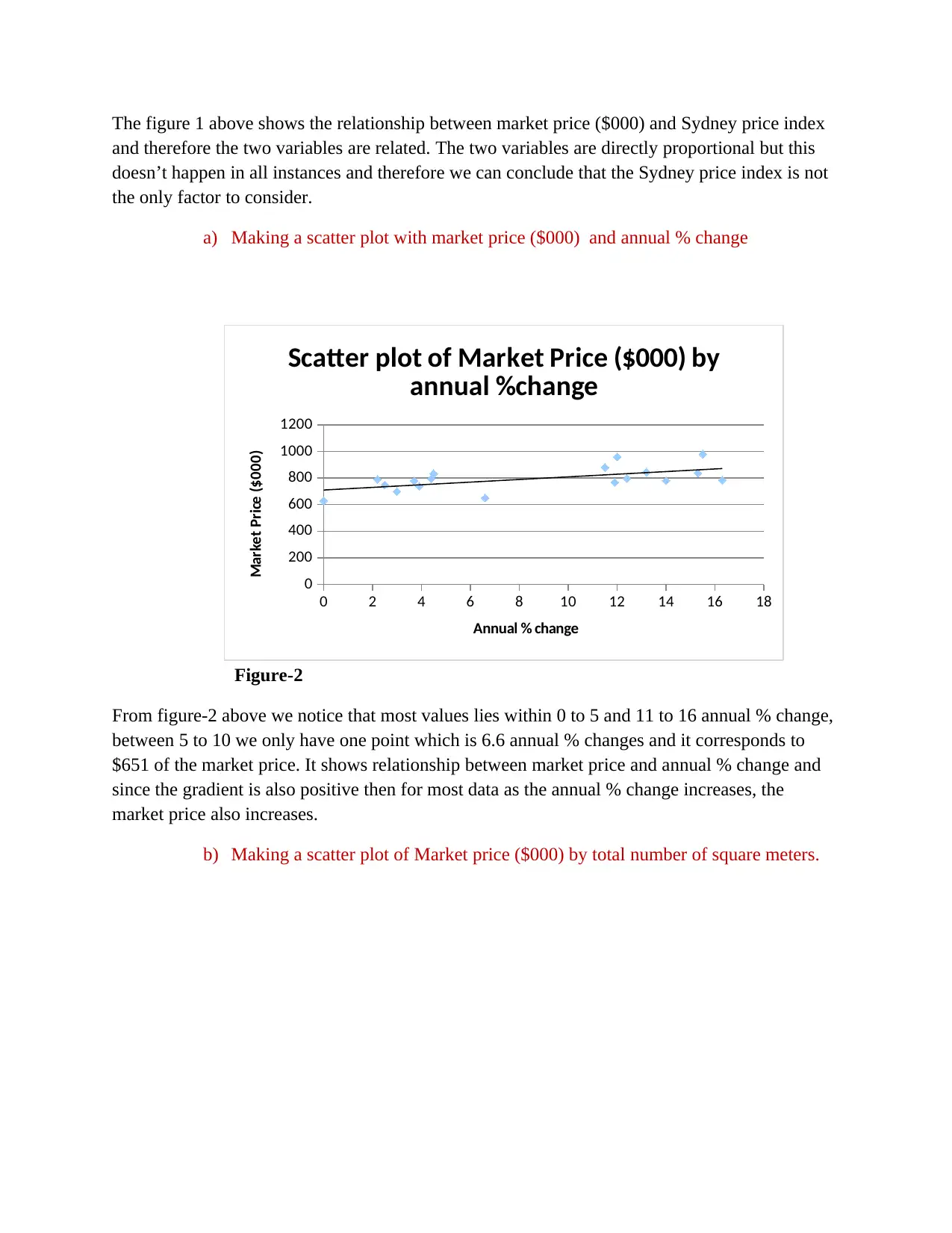
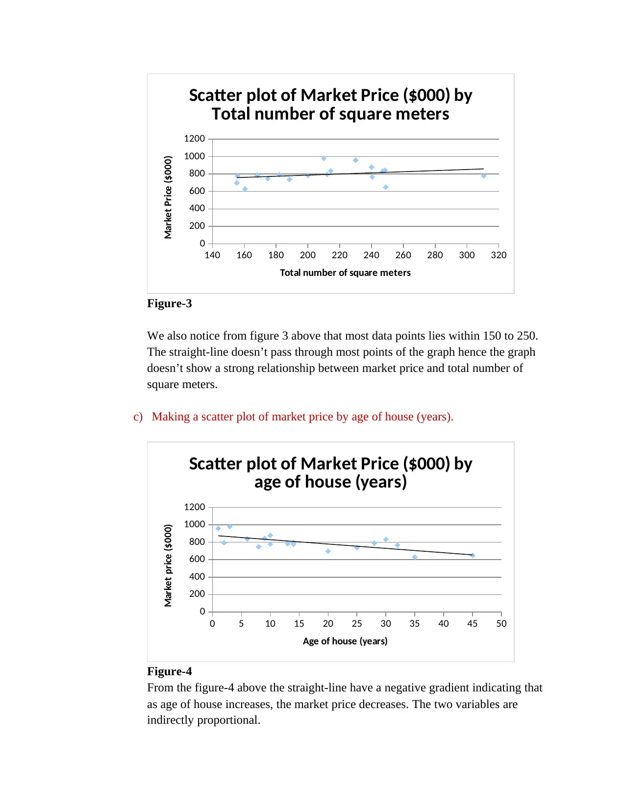
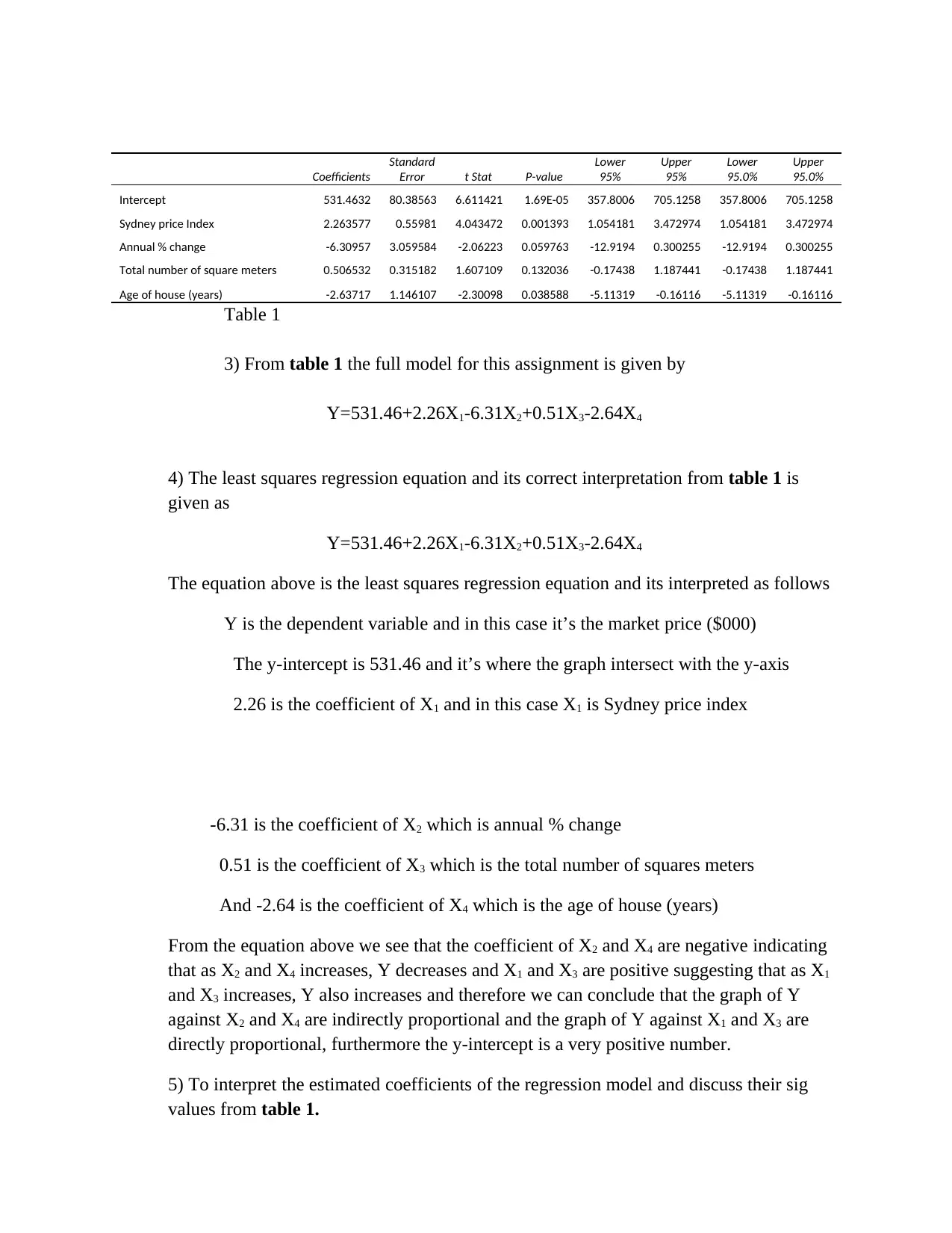
This case study analyzes the Sydney real estate market using multiple regression analysis. The assignment, for the STAT6003 course, explores the relationship between market prices and several independent variables including Sydney price index, annual percentage change, total number of square meters, and age of the house. The student develops and interprets an OLS regression model, examining coefficients, p-values, confidence intervals, and the coefficient of determination (R-squared) to assess the model's fit and the significance of each variable. The analysis includes scatter plots and interpretations of the relationships between variables. The study also compares the original model with re-estimated models, assessing how the removal of certain variables affects the overall explanatory power. The student also calculates and interprets the impact of total square meters on market price using the regression model. The student's analysis provides insights into the factors influencing house prices in the Sydney real estate market and the effectiveness of the regression models used. The student also provides an interpretation of the estimated coefficients of the regression model and discusses their sig values.

1) The OLS regression model of the form;
Y=β0+β1X1+β2X2+β3X3+β4X4+ε
The model above is used for estimating the unknown scalars that isβ0, β1, β2, β3, and β4
which are the coefficients of the independent variables. The sample size is part of the
population and therefore we only consider a sample size with five variables. In the
model above Y is the dependent variable and moreover, the independent variables are
variables that stand alone and don’t change by other variables. From the model above
the independent variables include X1, X2, X3 and X4. The unit of measurement of
these variables should always be considered as they help in understanding the model
better. The population is always very big hence analyzing all the data is always
expensive and time consuming and therefore we always consider the sample size
(Stock, James, Mark and Watson, 2015).
2)
60 80 100 120 140 160 180 200
0
200
400
600
800
1000
1200
Scatter plot of Market Price ($000) by
Sydney price index
Sydney price index
Market Price ($000)
Figure 1

The figure 1 above shows the relationship between market price ($000) and Sydney price index
and therefore the two variables are related. The two variables are directly proportional but this
doesn’t happen in all instances and therefore we can conclude that the Sydney price index is not
the only factor to consider.
a) Making a scatter plot with market price ($000) and annual % change
0 2 4 6 8 10 12 14 16 18
0
200
400
600
800
1000
1200
Scatter plot of Market Price ($000) by
annual %change
Annual % change
Market Price ($000)
FFigure-2
From figure-2 above we notice that most values lies within 0 to 5 and 11 to 16 annual % change,
between 5 to 10 we only have one point which is 6.6 annual % changes and it corresponds to
$651 of the market price. It shows relationship between market price and annual % change and
since the gradient is also positive then for most data as the annual % change increases, the
market price also increases.
b) Making a scatter plot of Market price ($000) by total number of square meters.

140 160 180 200 220 240 260 280 300 320
0
200
400
600
800
1000
1200
Scatter plot of Market Price ($000) by
Total number of square meters
Total number of square meters
Market Price ($000)
Figure-3
We also notice from figure 3 above that most data points lies within 150 to 250.
The straight-line doesn’t pass through most points of the graph hence the graph
doesn’t show a strong relationship between market price and total number of
square meters.
c) Making a scatter plot of market price by age of house (years).
0 5 10 15 20 25 30 35 40 45 50
0
200
400
600
800
1000
1200
Scatter plot of Market Price ($000) by
age of house (years)
Age of house (years)
Market price ($000)
Figure-4
From the figure-4 above the straight-line have a negative gradient indicating that
as age of house increases, the market price decreases. The two variables are
indirectly proportional.

Coefficients
Standard
Error t Stat P-value
Lower
95%
Upper
95%
Lower
95.0%
Upper
95.0%
Intercept 531.4632 80.38563 6.611421 1.69E-05 357.8006 705.1258 357.8006 705.1258
Sydney price Index 2.263577 0.55981 4.043472 0.001393 1.054181 3.472974 1.054181 3.472974
Annual % change -6.30957 3.059584 -2.06223 0.059763 -12.9194 0.300255 -12.9194 0.300255
Total number of square meters 0.506532 0.315182 1.607109 0.132036 -0.17438 1.187441 -0.17438 1.187441
Age of house (years) -2.63717 1.146107 -2.30098 0.038588 -5.11319 -0.16116 -5.11319 -0.16116
Table 1
3) From table 1 the full model for this assignment is given by
Y=531.46+2.26X1-6.31X2+0.51X3-2.64X4
4) The least squares regression equation and its correct interpretation from table 1 is
given as
Y=531.46+2.26X1-6.31X2+0.51X3-2.64X4
The equation above is the least squares regression equation and its interpreted as follows
Y is the dependent variable and in this case it’s the market price ($000)
The y-intercept is 531.46 and it’s where the graph intersect with the y-axis
2.26 is the coefficient of X1 and in this case X1 is Sydney price index
-6.31 is the coefficient of X2 which is annual % change
0.51 is the coefficient of X3 which is the total number of squares meters
And -2.64 is the coefficient of X4 which is the age of house (years)
From the equation above we see that the coefficient of X2 and X4 are negative indicating
that as X2 and X4 increases, Y decreases and X1 and X3 are positive suggesting that as X1
and X3 increases, Y also increases and therefore we can conclude that the graph of Y
against X2 and X4 are indirectly proportional and the graph of Y against X1 and X3 are
directly proportional, furthermore the y-intercept is a very positive number.
5) To interpret the estimated coefficients of the regression model and discuss their sig
values from table 1.

The model is given as follows
Y=531.46+2.26X1-6.31X2+0.51X3-2.64X4
From the model above its coefficients are;
531.46 is the y-intercept
2.26 is the coefficient of X1 (Sydney price index) and since its positive it indicates that as
X1 increases, Y also increases.
-6.31 is the coefficient of X2 (annual % change) and since its negative it indicates that as
X2 increases, Y decreases.
0.51 is the coefficient of X3 (total number of square meters) and since its positive it
indicates that as X3 increases, Y also increases.
-2.64 is the coefficient of X4 (age of house) and since its negative it indicates that as X4
increases, Y decreases.
The null hypothesis (H0) is that the y-intercept is statistically significant to the model.
The alternative hypothesis (H1) is that the y-intercept is not statistically significant to the
model.
The p-value is -0.41 which is less than 0.05
Therefore we fail to reject the null hypothesis and conclude that the y-intercept is
statistically significant to the model.
The null hypothesis (H0) is that the coefficient of X1 is statistically significant to the
model and the alternative hypothesis (H1) is that the coefficient of X1 is not statistically
significant to the model. The p-value is 0.001 which is less than 0.05 and hence we fail to
reject the null hypothesis and conclude that the coefficient of X1 is statistically significant
to the model.
The null hypothesis (H0) is that the coefficient of X2 is statistically significant to the
model and the alternative hypothesis (H1) is that this coefficient is not statistically
significant to the model. The p-value is 0.059 which is slightly greater than 0.05 hence
we reject the null hypothesis and conclude on the alternative hypothesis which state that
the coefficient is not statistically significant.
The null hypothesis (H0) states that the coefficient of X3 is statistically significant to the
model and the alternative hypothesis state that this coefficient is not statistically
significant to the model. The p-value is 0.13 which is greater than 0.05, hence we reject

the null hypothesis and conclude on the alternative hypothesis which state that the
coefficient has no significant difference to the model.
The null hypothesis states that the coefficient of X4 is statistically significant to the model
and the alternative hypothesis state that this coefficient is not statistically significant to
the model. The p-value is 0.038 which is less than 0.05 and therefore we fail to reject the
null hypothesis and conclude that the coefficient can be used for prediction in this model.
6) The value of the coefficient of determination for the relationship between the
dependent and independent variables and its interpretation from the table below.
Regression Statistics
Multiple R 0.899874
R Square 0.809773
The value of the coefficient of determination for the relationship between the dependent
and independent variable is 0.81 or 81%. This coefficient of determination measures the
extent that the dependent variable is predicted by the independent variable. The R-square
of 81% means that 81% of the dependent variable (market price) is predicted by the
independent variables. In this case the R-square is high indicating that the model is a
good fit for the data.
7) To state the 95% confidence intervals for each parameters and interpretations of the
intervals from table 1.
The confidence interval for y intercept is between 357.80 and 705.13 and therefore this
shows that the coefficient of y intercept can take any value within this range. The 95%
confidence interval for the coefficient of Sydney price index lies between 1.05 and 3.47
and this indicates that the coefficient can be any value within the given range (Mindrila
and Balentyne, 2013). Furthermore the 95% confidence interval for the coefficient of
total number of square meters also lies within -12.92 and 0.30 and therefore the
coefficient of annual % change can also be any value between the given ranges. The 95%
confidence interval for the coefficient of total number of square meters lies between -0.17
and 1.187 and any value within this range can be its coefficient. Last but not least the
95% confidence interval for the coefficient of age of house is between -5.11 and -0.16
and any value within this range can be the coefficient of age of house (years) (Moore,
Notz and Flinger, 2013).

8)
Regression Statistics
Multiple R
0.29630
6
R Square
0.08779
8
Adjusted R Square
0.03078
5
Standard Error
88.8269
9
Observations 18
Coefficients
Standard
Error t Stat P-value
Lower
95%
Upper
95%
Lower
95.0%
Upper
95.0%
Intercept 659.2613 110.9286 5.943113 2.06E-05 424.1031 894.4195 424.1031 894.4195
Total number of square meters 0.64259 0.51782 1.240953 0.232511 -0.45514 1.740319 -0.45514 1.740319
Table 2
The linear regression model from table 2 above is given as follows;
Y=659.26+0.643X
The value of the coefficient of determination for the relationship between the dependent
and independent variable is 8.8% or 0.088. This coefficient of determination measures
the extent that the dependent variable is predicted by the independent variable. The R-
square of 8.8% means that 8.8% of the dependent variable (market price) is predicted by
the independent variable (total number of square meters). The R-square value is small
indicating that the model is a poor fit for the data. The null hypothesis (H0) is that the
total number of square meters is statistically significant to this model. The alternative
hypothesis (H1) is that the total number of square meters is not statistically significant to
this model. The p-value is 0.23 which is greater than 0.05 and therefore we reject the null
hypothesis and conclude on the alternative hypothesis which states that the total number
of square meters is not statistically significant to the model. If we use this same test for
the y-intercept then we come into a conclusion that the y-intercept is statistically
significant for the model.
9) The original model from table 1 is given as
Y=531.46+2.26X1-6.31X2+0.51X3-2.64X4
R Square
0.68505
3

Coefficient
s
Standar
d Error t Stat P-value
Lower
95%
Upper
95%
Lower
95.0%
Upper
95.0%
Intercept 525.6761 47.19076 11.13939 6E-09 425.6361 625.716 425.6361 625.716
Sydney price Index 2.38858 0.404889 5.899344 2.24E-05 1.530254 3.246907 1.530254 3.246907
Table 3
And the re-estimated model from table 3 above for Sydney price index is
Y=525.68+2.39X1
The R-square for the original model is 81% and that for the re-estimated model is 69%
and these coefficients of determination are high we can conclude that the models are
good fit for the data.
R
Square
0.1986
57
Coefficients
Standard
Error t Stat P-value
Lower
95%
Upper
95%
Lower
95.0%
Upper
95.0%
Intercept 732.395 36.82037 19.89103 1.04E-12 654.3393 810.4507 654.3393 810.4507
Annual % change 7.304704 3.66775 1.991603 0.063769 -0.47058 15.07999 -0.47058 15.07999
Table 5
Using the re-estimated model from table 5 for annual % change whose model is given as
Y=732.40+7.30X2
When this is compared with the original model we notice that the R-square is 20% hence
this value is low and we conclude that the model is a poor fit for the data. The model
from table 2 for total number of square meters is given by
Y=659.26+0.643X3
Its R-square is 8.8% which is very low hence not good fit for the data.
R Square
0.49657
4
Coefficients
Standard
Error t Stat P-value
Lower
95%
Upper
95%
Lower
95.0%
Upper
95.0%
Intercept 878.8293 26.32692 33.3814 3.19E-16 823.0187 934.6399 823.0187 934.6399
Age of house (years) -4.98009 1.253584 -3.97268 0.001093 -7.63757 -2.32261 -7.63757 -2.32261
Table 4
Finally from table 4 the model for age of house is given by

Y=878.83-4.98X4
Its R-square is 50% which is still low hence not good fit for the data.
10) The model from table 2 is given as
Y=659.26+0.643X3
Now replacing X3 with 400 from the model above we get
Y=659.26+0.643(400)
=$916

References
Stock, James H. and Mark W. Watson (2015), Introduction to Economet-rics, 3rd ed., Pearson
Addison-Wesley. Chapters 4 - 9.
Moore, D. S., Notz, W. I, & Flinger, M. A. (2013). The basic practice of statistics(6thed.). New
York, NY: W. H. Freeman and Company.
Mindrila, D. and Balentyne, P. (2013). [online] Westga.edu. Available at:
https://www.westga.edu/academics/research/vrc/assets/docs/confidence_intervals_not
es.pdf [Accessed 6 May 2019].