Hydraulic Design Calculations for a Gravity Driven Piping System

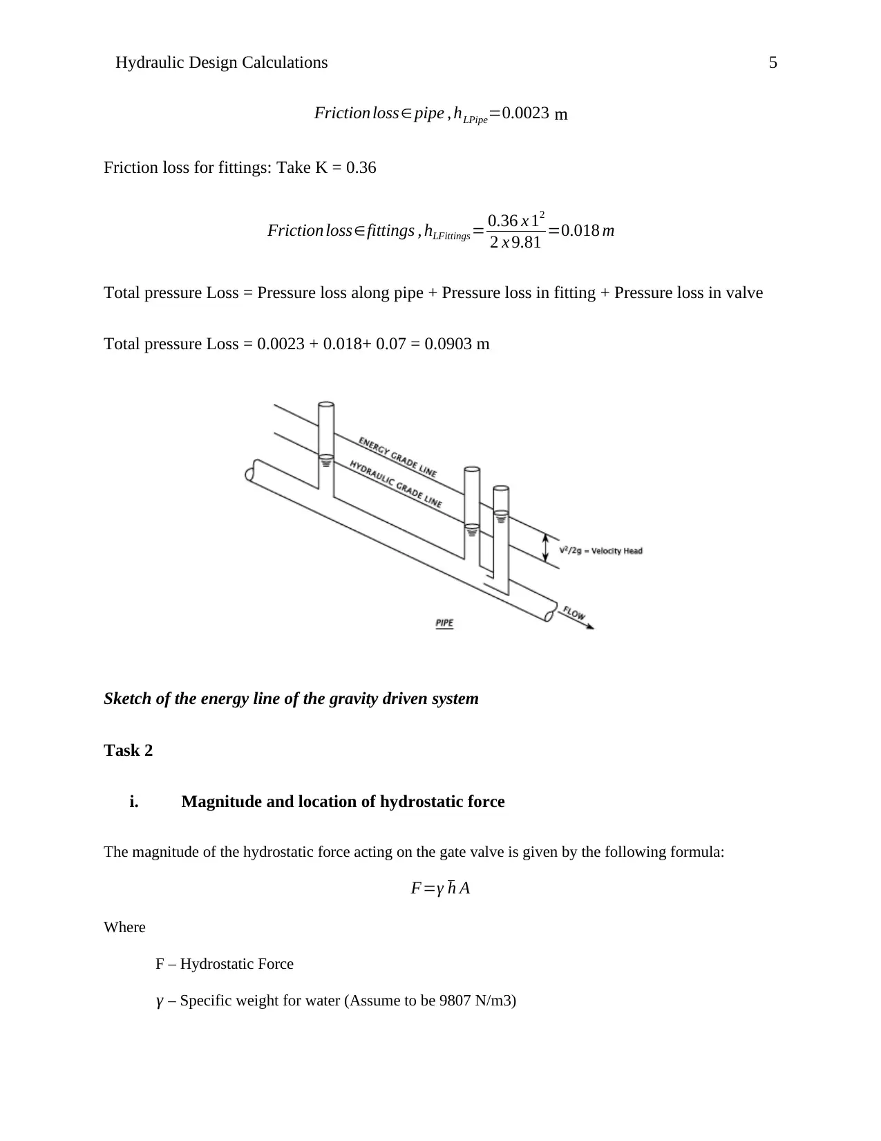
This document presents hydraulic design calculations for a gravity-driven piping system. It includes determining the pipe diameter, selecting appropriate pipe material (HDPE PN25), calculating the gradient using the Hazen-Williams formula, and computing pipe friction coefficient and losses. The analysis extends to hydrostatic force magnitude and location on a gate valve, resultant force at a 90-degree bend, and determining the depth, width, and bed slope of a rectangular channel using Manning's equation. Furthermore, it calculates the additional mass needed for a buoy and the total volume of concrete required for channel construction. The document also incorporates a sketch of the energy line for the gravity-driven system.

Hydraulic Design Calculations 1
Hydraulic Design for Gravity driven Piping System
By
Student Name
Name of Class
Professsor
Name of Institution
(Date)

Hydraulic Design Calculations 2
Task 1
Compute the following
i. Diameter of the pipe
Give the following:
V =1.0 m
s ; Q=355 l
s ; H=14.2 m; L 1=1450 m; L 2=6300 m; Bd=0.81 m; Bh=1.25 m;
Bm=45.5 kg
The discharge is calculated using the following formula:
Q= Area x velocity= π d2
4 x v
Then substituting for all the known values:
d2= Q 4
πv = 4 x 0.355
3.142 x 1
The diameter is then found to be
d=0.452m
d=452 mm ≈ 500mm
The standard pipe to be used in this scenario will be 500 mm diameter pipe.
ii. Pipe material
The pipe material selected for this case will be High density polyethylene (HDPE) pipe.
Considering a head of 14.2 m, the expected pressure in the pipes would be 142 bar. Considering

Hydraulic Design Calculations 3
a safety factor of 1.5, the maximum pressure expected in the system would be 213 bar.
Therefore, the pipe to be selected would be HDPE PN25.
iii. Gradient
Using the Hazen Williams Formula, the gradient of the pipe would be:
Gradient=162,000,00 x (Design flow / HWC)1.85 x( Internal Diameter
10 )
−4.87
Where
Gradient - m/km
Diameter to be internal in mm (Given as 500 mm)
Hazen William Coefficient (140 for plastic pipes)
Design Flow in l/s ( Given as 355 l/s)
Therefore:
Gradient=162,000,00 x (355/140)1.85 x ( 500
10 )
−4.87
Gradient=4.2m/km
iv. Compute pipe friction coefficient, λ and friction losses
Frictional losses along the pipe and fittings can be calculated using the following formulas:
Friction loss∈pipe , hLPipe=4 λLV 2
D2 g
Friction loss∈fittings , hLFittings=∑ KFittings V 2
2 g

Hydraulic Design Calculations 4
Where
V - Velocity
D - Inner diameter of pipe
L - Pipe Length
g – Gravity
K - Resistance coefficient for fittings
λ - Pipe friction coefficient
hL - Pressure drop;
To determine the kind of flow we would have, we compute the Re number:
ℜ=ρ cd
μ
Where
ρ – Density of water = 1000 kg/m3
c – Velocity (Given 1 m/s)
μ - coefficient of dynamic viscosity (Given as 1.4 x 10-3 NS/m2)
d – Diameter (given as 500mm)
Therefore:
ℜ=1000 x 1 x 0.5
1.14 x 10−3
ℜ=438596; Therefore the flow is turbulent
For the turbulent flow, the λ - Pipe friction coefficient will be calculated using the Blasius equation:
f = 0.079
ℜ1 / 4 = 7.204 x 10-7
Friction loss in pipe is given by:
Friction loss∈ pipe , hLPipe=4 x 7.204 x 10−7 x 7750 x 12
0.5 x 2 x 9.81

Hydraulic Design Calculations 5
Friction loss∈ pipe , hLPipe=0.0023 m
Friction loss for fittings: Take K = 0.36
Friction loss∈fittings , hLFittings= 0.36 x 12
2 x 9.81 =0.018 m
Total pressure Loss = Pressure loss along pipe + Pressure loss in fitting + Pressure loss in valve
Total pressure Loss = 0.0023 + 0.018+ 0.07 = 0.0903 m
Sketch of the energy line of the gravity driven system
Task 2
i. Magnitude and location of hydrostatic force
The magnitude of the hydrostatic force acting on the gate valve is given by the following formula:
F=γ h A
Where
F – Hydrostatic Force
γ – Specific weight for water (Assume to be 9807 N/m3)

Hydraulic Design Calculations 6
A – Cross sectional Area of the gate valve
h - The vertical distance of the centroid below the water surface
To get the Area of the gate valve:
Area= π d2
4 = π x 0.52
4 =0.196375 m 2
The vertical distance of the centroid below the water surface:
h= ( H + y )= (14.2+ 0.5
2 )=14.45 m
Force is then given by:
F=9807 x 14.45 x 0.196375
F=27.829 kN
The location of centre of pressure is then given by:
y p= I o
A y + y
Where
I o – Moment of inertia about the neutral x axis
I o= 1
64 x d4 = 1
64 x 0.54 =3.06836 x 10−3 m 4
y p= 3.06836 x 10−3
0.196375 x 14.45 +14.45=14.4512 mbelow the water surface
ii. Magnitude and direction of resultant force at 90o bend
The resultant force will be given by the formula:
Force=mass flow rate x velocity=m x v=ρ x A x V 2
mass flow rate=ρ x A x V =1000 x 0.196375 x 1=196.375 kg/ s
Force=196.375 x 1=196.375 N

Hydraulic Design Calculations 7
The resultant force will act opposite to the direction of flow of water in the pipe.
Task 3
3.1 To determine the depth, width and bed slope of the rectangular channel:
Using the manning equation
v= 1
n x R
2
3 x S
1
2
Where
V – is velocity given as 1 m/s
Manning’s coefficient, n to be 0.013 m-1/3/s
R – Hydraulic radius
S - Slope of channel
Given the discharge Q = 355 l/s or 0.355 m3/s
Take the width of the channel to be, b = 0.5m
To get the depth, y of the channel:
Q= Area x Velocity= AxV
Q= y x b x v
0.355= y x 0.5 x 1
y=0.71m∨710 mm depth
To get the slope, we will apply the Using the manning equation

Hydraulic Design Calculations 8
v= 1
n x R
2
3 x S
1
2
Give: n = 0.013 m-1/3/s, v = 1 m/s, first we calculate R:
R= Area
Wetted Perimeter
R= b x y
b+ 2 y
R= 0.51+0.71
0.71+2( 0.71)=0.5728 m
Substituting all the components into the manning’s equation:
1= 1
0.013 x 0.5728
2
3 x S
1
2
Making S1/2 the subject:
S
1
2 =( 1/1
0.013 x 0.5728
2
3 )
Calculating for the value of S:
S = 0.036%
3.2
Given the dimensions:
Bd=0.81 m; Bh=1.25 m; Bm=45.5 kg
Considering the freeboard of 0.25 m; then the height to be submerged will be 1 m.
Find the area of the buoy:

Hydraulic Design Calculations 9
Area= π d2
4 = π x 0.812
4 =0.515 m 2
To find the volume:
Volume=Area x submerged height
Volume=0.515 x 1=0.515m 3
As per the Archimedes principle, the buoy floating on water will displace volume of water equal
to its own volume. Therefore, the volume of water displaced is 0.515 m3.
To get the mass of water that is displaced: Taking the density of water to be 1000 kg/m3
Mass=density x volume
Mass=1000 x 0.515=515 kg
Therefore, the additional mass to be added to the buoy:
Maximum mass = 515 – 45.5 = 469.5 kg
3.3
Total volume of concrete
Given: wall thickness = 0.1m; width = 0.5 m; depth = 0.71 m; channel length = 50m;
Volume = Cross sectional area x length of channel
= (2(0.1x0.71) + (0.5x0.1)) x 50
= 9.6 m3 of concrete would be used to make the channel.
Total area of formwork

Hydraulic Design Calculations 10
Area = 4 x (0.71x50) + (0.5x50) = 167 m2

Hydraulic Design Calculations 11
Bibliography
d'Almeida, A. (2008). Transition of unsteady flows of evaporation to steady state. Comptes
Rendus Mécanique, 336(7), pp.612-615.
Delplace, F. (2016). Fluid Mechanics at Atomic Scale. Fluid Mechanics: Open Access, 03(02).
Douglas, J. (2011). Fluid mechanics. Harlow: Prentice Hall.
Garde, R. (2010). Turbulent flow. Tunbridge Wells, UK: New Age Science Limited.
Granger, R. (2012). Fluid Mechanics. Dover Publications.
Jones, R. (2014). Principles of non-newtonian fluid mechanics. Journal of Non-Newtonian Fluid
Mechanics, 1(1), p.106.
Landau, L. and Lifšic, E. (2011). Fluid mechanics. Amsterdam [u.a]: Elsevier/Butterworth
Heinemann.
Munson, B. (2013). Fluid mechanics. Singapore: John Wiley & Sons.

Hydraulic Design Calculations 12