Hydro Design Project: Comparing Flood Estimation Methods and Design

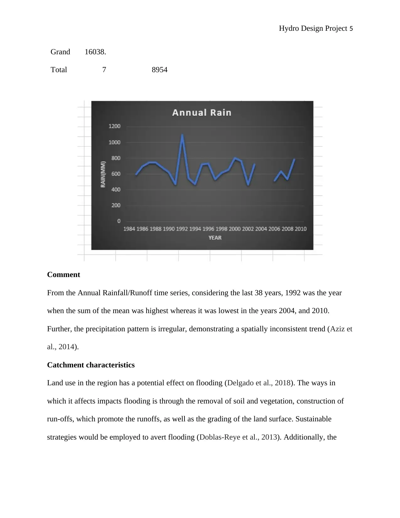
This hydro design project analyzes various aspects of hydrology and flood estimation. It begins with a seasonality plot and rainfall/runoff time series analysis, identifying wet and dry seasons and highlighting years with extreme rainfall. The project then addresses the impact of missing data in annual peak flow series, proposing strategies to minimize its effects. It further explores catchment characteristics and land use impacts on flooding. The core of the project involves estimating flood quantiles using different methods including FLIKE and Regional Flood Frequency Estimation (RFFE), and probabilistic rational method. The project uses ARR data and catchment characteristics like latitude, longitude, and catchment area. The project concludes by comparing the design flow estimates obtained from different methods, including their operating principles and levels of uncertainty. The analysis recommends the Flood Frequency Analysis with FLIKE due to its ability to fit the data, leading to minimal uncertainty.

Hydro Design Project 1
HYDRO DESIGN PROJECT
Name of student
Institution
Date

Hydro Design Project 2
Task 1
SEASONALITY PLOT
Row
Labels Average of Total Month
Avg of
monthly(mm/month)
1 0.607355 1 0.61
2 0.744901 2 0.74
3 0.730581 3 0.73
4 1.506533 4 1.51
5 2.311942 5 2.31
6 2.958136 6 2.96
7 3.288483 7 3.29
8 2.809293 8 2.81
9 2.511277 9 2.51
10 1.851421 10 1.85
11 1.139067 11 1.14
12 1.233721 12 1.23
Grand
Total 1.791233

Hydro Design Project 3
Comment
Considering the average monthly rainfall, the region is divided into a wet season from March to
October, and a dry season from November to February, with a peak-wet season in the month of
July.
Annual Rainfall/Runoff time series
Row
Labels
Sum of
Total Count of Total Year
Annual
Rain(mm/year
)
1984 106 109 1984
1985 596.1 365 1985 596.1
1986 699 365 1986 699
1987 748.3 365 1987 748.3
1988 750.2 366 1988 750.2

Hydro Design Project 4
1989 686.3 365 1989 686.3
1990 624.3 365 1990 624.3
1991 475.4 363 1991 475.4
1992 1095.2 366 1992 1095.2
1993 550 365 1993 550
1994 477.4 365 1994 477.4
1995 724.4 365 1995 724.4
1996 734.4 365 1996 734.4
1997 535 365 1997 535
1998 616.2 364 1998 616.2
1999 656.5 365 1999 656.5
2000 803 366 2000 803
2001 767.6 365 2001 767.6
2002 469.6 365 2002 469.6
2003 721 365 2003 721
2004 88.4 139 2004
2005 377.4 135 2005
2006 517.8 365 2006 517.8
2007 637.6 360 2007 637.6
2008 537.4 366 2008 537.4
2009 787.6 365 2009 787.6
2010 256.6 180 2010

Hydro Design Project 5
Grand
Total
16038.
7 8954
Comment
From the Annual Rainfall/Runoff time series, considering the last 38 years, 1992 was the year
when the sum of the mean was highest whereas it was lowest in the years 2004, and 2010.
Further, the precipitation pattern is irregular, demonstrating a spatially inconsistent trend (Aziz et
al., 2014).
Catchment characteristics
Land use in the region has a potential effect on flooding (Delgado et al., 2018). The ways in
which it affects impacts flooding is through the removal of soil and vegetation, construction of
run-offs, which promote the runoffs, as well as the grading of the land surface. Sustainable
strategies would be employed to avert flooding (Doblas‐Reye et al., 2013). Additionally, the

Hydro Design Project 6
removal of vegetation will likely increase the surface runoff, and impacting flooding. Trees
should be planted to help in the interception process (Eisner et al., 2017).

Hydro Design Project 7
Task 2
With reference to the below annual series data and graphs, it is noted that the years with missing
daily data are 1991, 2004 and 2005 as highlighted in blue in the data table above. The various
strategies in which the impact of missing data on the annual series of peak flows can be
minimized include:
 Only the observation gauges having less than 15% missing data in the period 1990 to 2006 were
to be identified (Evin et al., 2016)
 They then need to be filtered to obtain GEV fit followed by simulation
Annual time series of the peak flows
Row
Labels
Sum of
Mean Count of Mean2 Year
Annual
Flow(ML/year)
Annual
Flow(m^3/year)
Annual
Flow(mm/year)
1972 430.857 228 1972
1973 1298.427 365 1973 1298.427 1298427 154574642.9
1974 2661.945 365 1974 2661.945 2661945 316898214.3
1975 927.613 365 1975 927.613 927613 110430119
1976 103.209 366 1976 103.209 103209 12286785.71
1977 161.227 365 1977 161.227 161227 19193690.48
1978 1198.246 365 1978 1198.246 1198246 142648333.3
1979 1159.003 365 1979 1159.003 1159003 137976547.6
1980 238.351 366 1980 238.351 238351 28375119.05
1981 2537.722 365 1981 2537.722 2537722 302109761.9
1982 9.139 365 1982 9.139 9139 1087976.19

Hydro Design Project 8
1983 879.602 365 1983 879.602 879602 104714523.8
1984 702.394 366 1984 702.394 702394 83618333.33
1985 282.489 365 1985 282.489 282489 33629642.86
1986 797.306 365 1986 797.306 797306 94917380.95
1987 1232.016 365 1987 1232.016 1232016 146668571.4
1988 1112.897 366 1988 1112.897 1112897 132487738.1
1989 1029.479 365 1989 1029.479 1029479 122557023.8
1990 908.438 365 1990 908.438 908438 108147381
1991 370.896 327 1991
1992 3275.921 366 1992 3275.921 3275921 389990595.2
1993 140.14 365 1993 140.14 140140 16683333.33
1994 5.461 365 1994 5.461 5461 650119.0476
1995 1107.558 365 1995 1107.558 1107558 131852142.9
1996 1481.225 366 1996 1481.225 1481225 176336309.5
1997 18.813 365 1997 18.813 18813 2239642.857
1998 137.105 365 1998 137.105 137105 16322023.81
1999 39.602 365 1999 39.602 39602 4714523.81
2000 1065.168 366 2000 1065.168 1065168 126805714.3
2001 1086.075 365 2001 1086.075 1086075 129294642.9
2002 1.162 365 2002 1.162 1162 138333.3333
2003 518.607 365 2003 518.607 518607 61738928.57
2004 0 139 2004
2005 1038.25 130 2005

Hydro Design Project 9
2006 95.621 365 2006 95.621 95621 11383452.38
2007 175.98 365 2007 175.98 175980 20950000
2008 43.915 366 2008 43.915 43915 5227976.19
2009 982.783 365 2009 982.783 982783 116997976.2
2010 0 116 2010
Grand
Total 29254.642 13358
Comment
From the data and graph, above, the annual rain was at peak in the year 1992, while other years
were averagely the same. However, there were missing data in the years 1991, 2004 and 2005,
resulting in a significant effect in the years.

Hydro Design Project 10
Lognormal probability plot
-2 2
AEP 1 in Y
-3.00
-0.80
1.40
3.60
5.80
8.00
log10(Peak flow m^3/s)
1.5 2 5 10 20 50 100
Gauged
Expected quantile
90% limit
Expected prob quantile

Hydro Design Project 11
Comment
From the probability plots, there was a trend observed around the model for two sets of data.
Both combinations of the data set displayed the least-squares regression (Haddad and Rahman,
2014), hence, the model was appropriate for the data and that the lognormal distribution was a
more appropriate choice.

Hydro Design Project 12
Task 3
Datetime: 2020-04-04 19:42
Region name: Humid SA
Region code: 3
Site name: A5030508 Inverbrackie/Craigbk
Latitude at catchment outlet (degree) = -34.9472
Longitude at catchment outlet (degree) = 138.9256
Latitude at catchment centroid (degree) = -34.939
Longitude at catchment centroid (degree) = 138.9519
Distance of the nearest gauged catchment in the database (km) = 0.51
Catchment area (sq km) = 8.4
Design rainfall intensity, 1 in 2 AEP and 6 hr duration (mm/h): 5.181941
Design rainfall intensity, 1 in 50 AEP and 6 hr duration (mm/h): 11.485929
Shape factor of the ungauged catchment: 0.88
ESTIMATED FLOOD QUANTILES:
AEP (%) Expected quantiles (m^3/s) 5% CL m^3/s 95% CL m^3/s
50 1.00 0.300 3.31
20 1.80 0.580 5.69
10 2.46 0.780 7.83
5 3.18 0.950 10.5
2 4.25 1.17 14.8