A Null and Alternative Hypothesis Test on Student Weights, Mumbai Uni

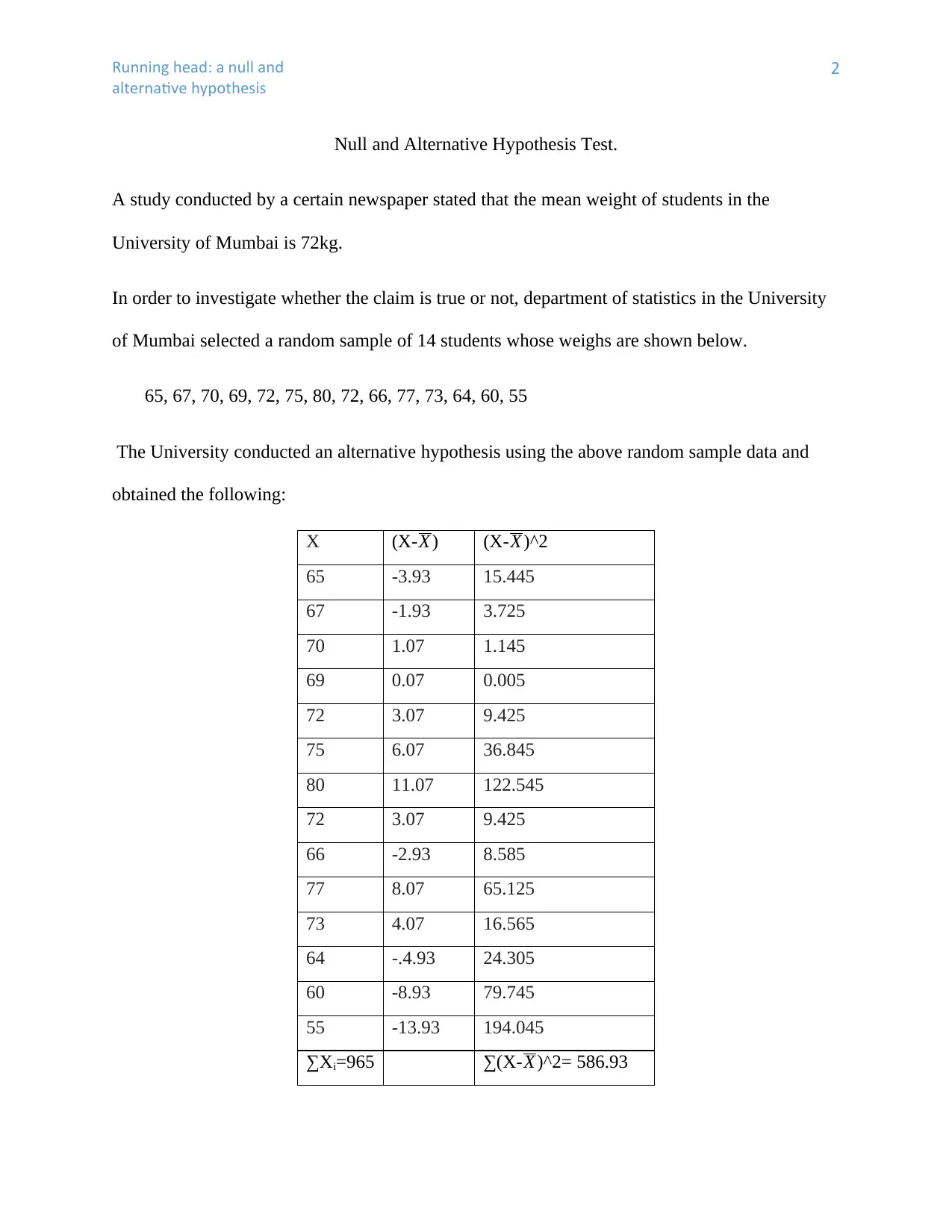
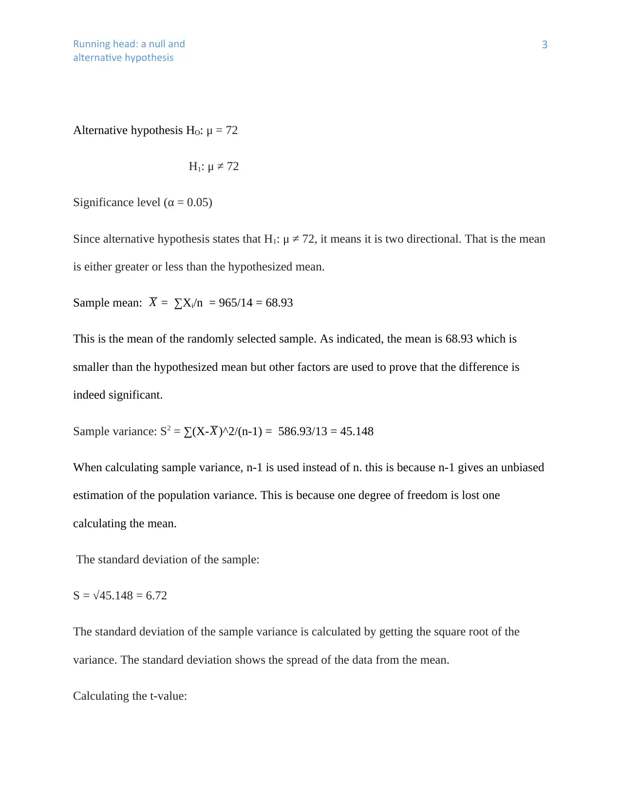
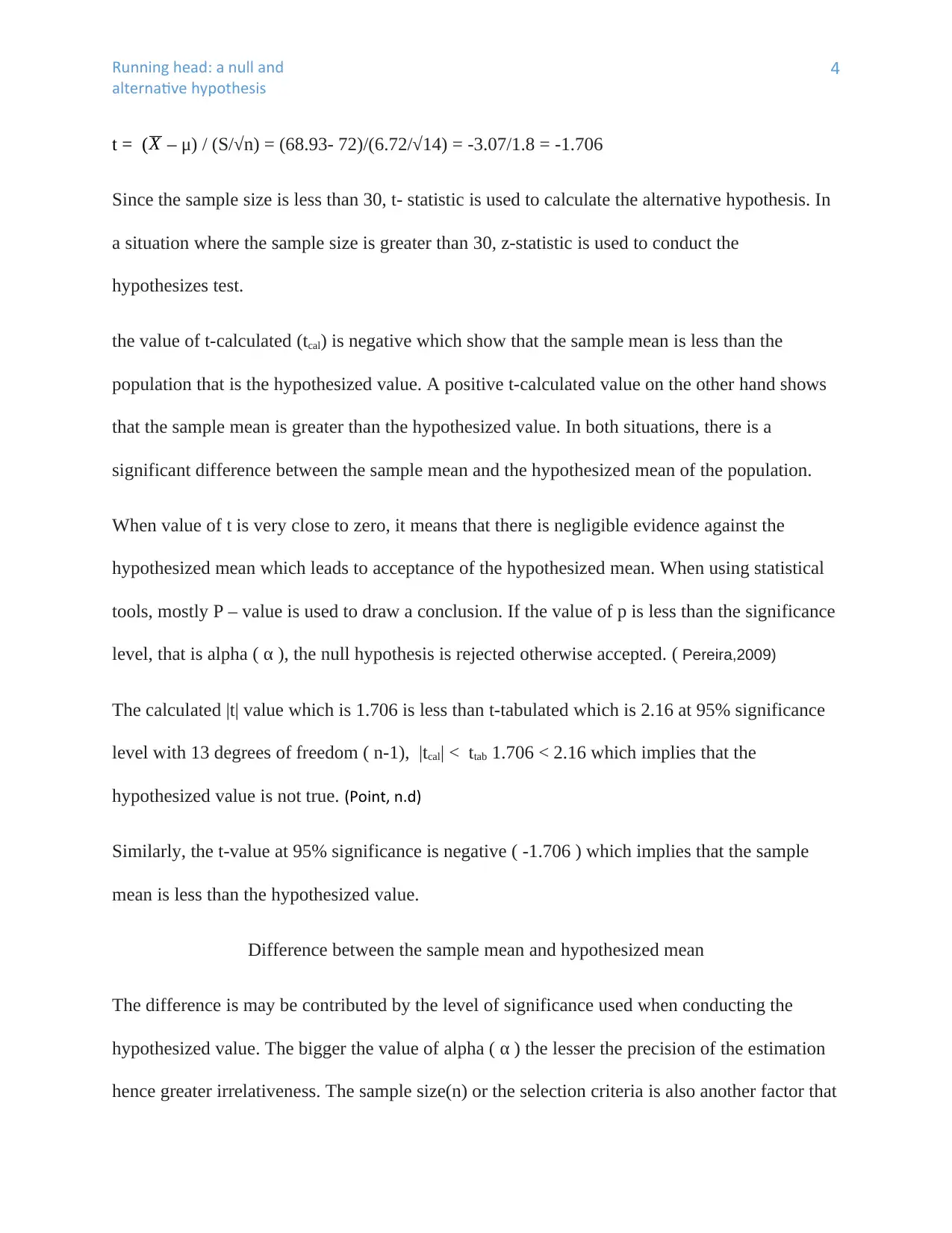
This report presents a null and alternative hypothesis test conducted to investigate the claim that the mean weight of students at the University of Mumbai is 72kg. A random sample of 14 students' weights was collected, and statistical analysis was performed, including calculating the sample mean, variance, standard deviation, and t-value. The calculated t-value was compared to the t-tabulated value to determine whether to reject or accept the null hypothesis. The report discusses potential reasons for differences between the sample mean and hypothesized mean, such as the significance level and sample size. The conclusion indicates that there is sufficient evidence to reject the hypothesized value at a 95% significance level, acknowledging the possibility of Type I and Type II errors. Desklib provides access to this and similar solved assignments for students.

Running head: a null and
alternative hypothesis
1
Null and Alternative hypothesis test
Name:
Instructor:
Affiliated institution:

Running head: a null and
alternative hypothesis
2
Null and Alternative Hypothesis Test.
A study conducted by a certain newspaper stated that the mean weight of students in the
University of Mumbai is 72kg.
In order to investigate whether the claim is true or not, department of statistics in the University
of Mumbai selected a random sample of 14 students whose weighs are shown below.
65, 67, 70, 69, 72, 75, 80, 72, 66, 77, 73, 64, 60, 55
The University conducted an alternative hypothesis using the above random sample data and
obtained the following:
X (X-X ) (X-X )^2
65 -3.93 15.445
67 -1.93 3.725
70 1.07 1.145
69 0.07 0.005
72 3.07 9.425
75 6.07 36.845
80 11.07 122.545
72 3.07 9.425
66 -2.93 8.585
77 8.07 65.125
73 4.07 16.565
64 -.4.93 24.305
60 -8.93 79.745
55 -13.93 194.045
∑Xi=965 ∑(X-X )^2= 586.93

Running head: a null and
alternative hypothesis
3
Alternative hypothesis HO: μ = 72
H1: μ ≠ 72
Significance level (α = 0.05)
Since alternative hypothesis states that H1: μ ≠ 72, it means it is two directional. That is the mean
is either greater or less than the hypothesized mean.
Sample mean: X = ∑Xi/n = 965/14 = 68.93
This is the mean of the randomly selected sample. As indicated, the mean is 68.93 which is
smaller than the hypothesized mean but other factors are used to prove that the difference is
indeed significant.
Sample variance: S2 = ∑(X- X )^2/(n-1) = 586.93/13 = 45.148
When calculating sample variance, n-1 is used instead of n. this is because n-1 gives an unbiased
estimation of the population variance. This is because one degree of freedom is lost one
calculating the mean.
The standard deviation of the sample:
S = √45.148 = 6.72
The standard deviation of the sample variance is calculated by getting the square root of the
variance. The standard deviation shows the spread of the data from the mean.
Calculating the t-value:

Running head: a null and
alternative hypothesis
4
t = ( X – μ) / (S/√n) = (68.93- 72)/(6.72/√14) = -3.07/1.8 = -1.706
Since the sample size is less than 30, t- statistic is used to calculate the alternative hypothesis. In
a situation where the sample size is greater than 30, z-statistic is used to conduct the
hypothesizes test.
the value of t-calculated (tcal) is negative which show that the sample mean is less than the
population that is the hypothesized value. A positive t-calculated value on the other hand shows
that the sample mean is greater than the hypothesized value. In both situations, there is a
significant difference between the sample mean and the hypothesized mean of the population.
When value of t is very close to zero, it means that there is negligible evidence against the
hypothesized mean which leads to acceptance of the hypothesized mean. When using statistical
tools, mostly P – value is used to draw a conclusion. If the value of p is less than the significance
level, that is alpha ( α ), the null hypothesis is rejected otherwise accepted. ( Pereira,2009)
The calculated |t| value which is 1.706 is less than t-tabulated which is 2.16 at 95% significance
level with 13 degrees of freedom ( n-1), |tcal| < ttab 1.706 < 2.16 which implies that the
hypothesized value is not true. (Point, n.d)
Similarly, the t-value at 95% significance is negative ( -1.706 ) which implies that the sample
mean is less than the hypothesized value.
Difference between the sample mean and hypothesized mean
The difference is may be contributed by the level of significance used when conducting the
hypothesized value. The bigger the value of alpha ( α ) the lesser the precision of the estimation
hence greater irrelativeness. The sample size(n) or the selection criteria is also another factor that

Running head: a null and
alternative hypothesis
5
may contribute to the difference of the sample mean and hypothesized mean of the population.
The larger the size of the sample the better the results. (Lane, 2011)
Comparison between the sample and population characteristics
The characteristics of the randomly selected sample are similar to that of the population which
the sample is drawn from. There is no geographical difference since both the population and the
sample are students of the University of Mumbai hence live in the same area. Since the sample is
randomly selected from the students of the University of Mumbai, economic, cultural or social
differences of the students are treated to be insignificant to contribute to their weight because the
sample itself represents that diversity.
Decision rule:
Reject the null hypothesis. this decision has arrived since the t-value calculated is negative and
not very close to zero.
Conclusion
Since t-calculated value is negative, it means the sample mean is less than the hypothesized value
and therefore, there is sufficient evidence to reject the hypothesized value under a 95%
significance level. A significance level of 0.05 is close to accurate hence leads to commendable
decisions.
Based on this decision, type I error (alpha- α) may be committed by rejecting Ho while it’s
actually true. This the probability (alpha) of rejecting Ho while it is true. On the other hand, type II
error is committed by failing to reject the null hypothesis while it is actually false. This is the
probability beta (β) of accepting the null hypothesis while it is supposed to be rejected.

Running head: a null and
alternative hypothesis
6
References
Lane, D. M. (2011, 08 05). Statistical Power. Retrieved from Wikieducator:
http://wikieducator.org/Statistical_power
Point, T. (n.d). Statistics-T test. Retrieved from tutorials point:
https://www.tutorialspoint.com/statistics/student_t_test.htm
Pereira, S. M., & Leslie, G. (2009). Hypothesis testing. Australian Critical Care, 22(4), 187-191.