ITEC 6401 - Hypothesis Testing Assignment on Wage Dataset Analysis

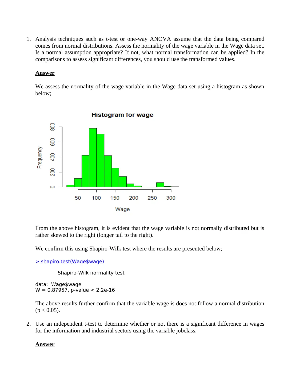
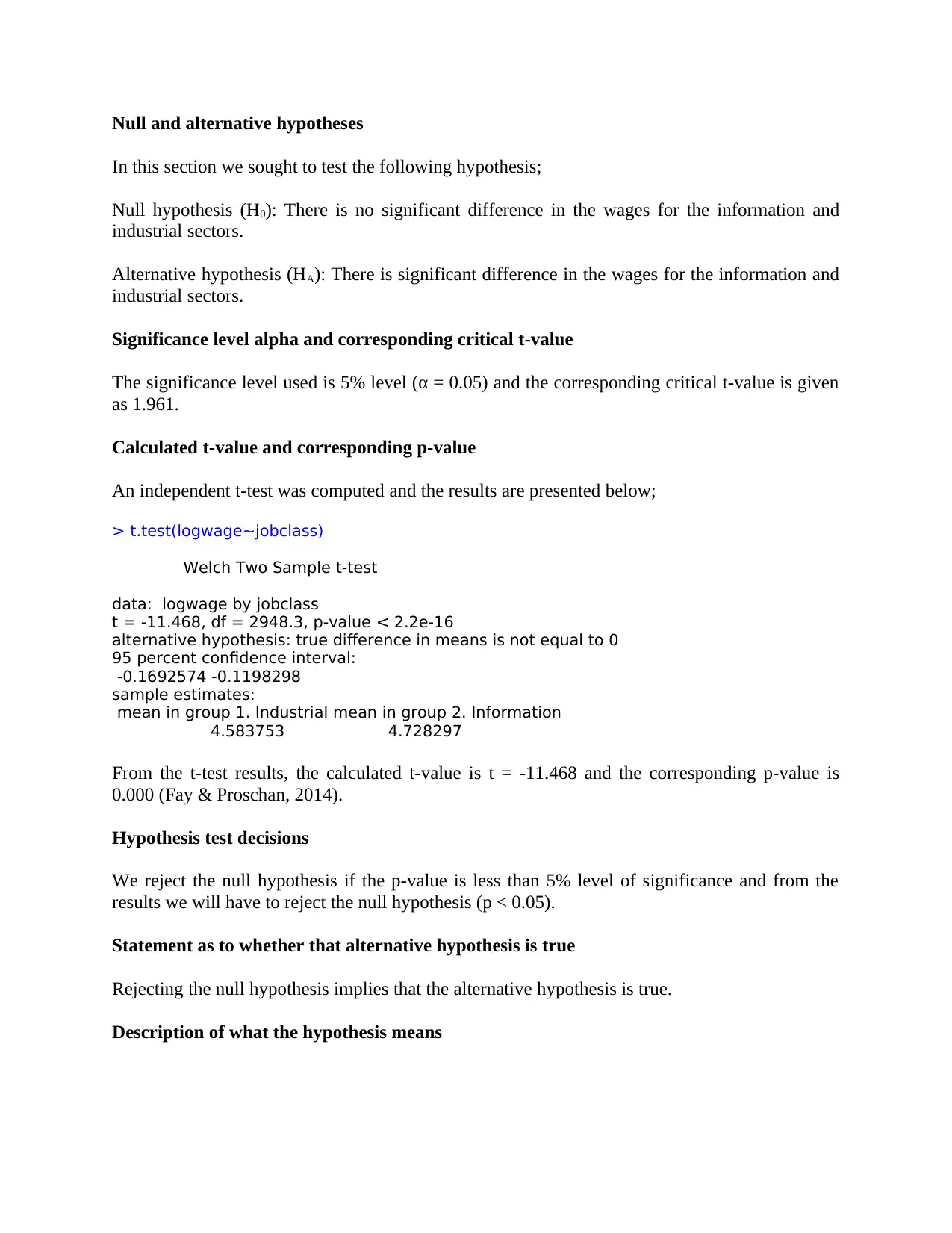
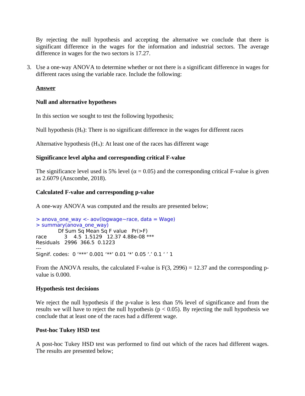
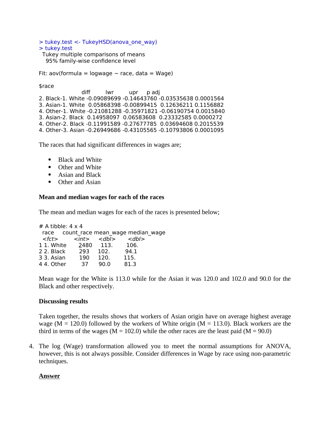
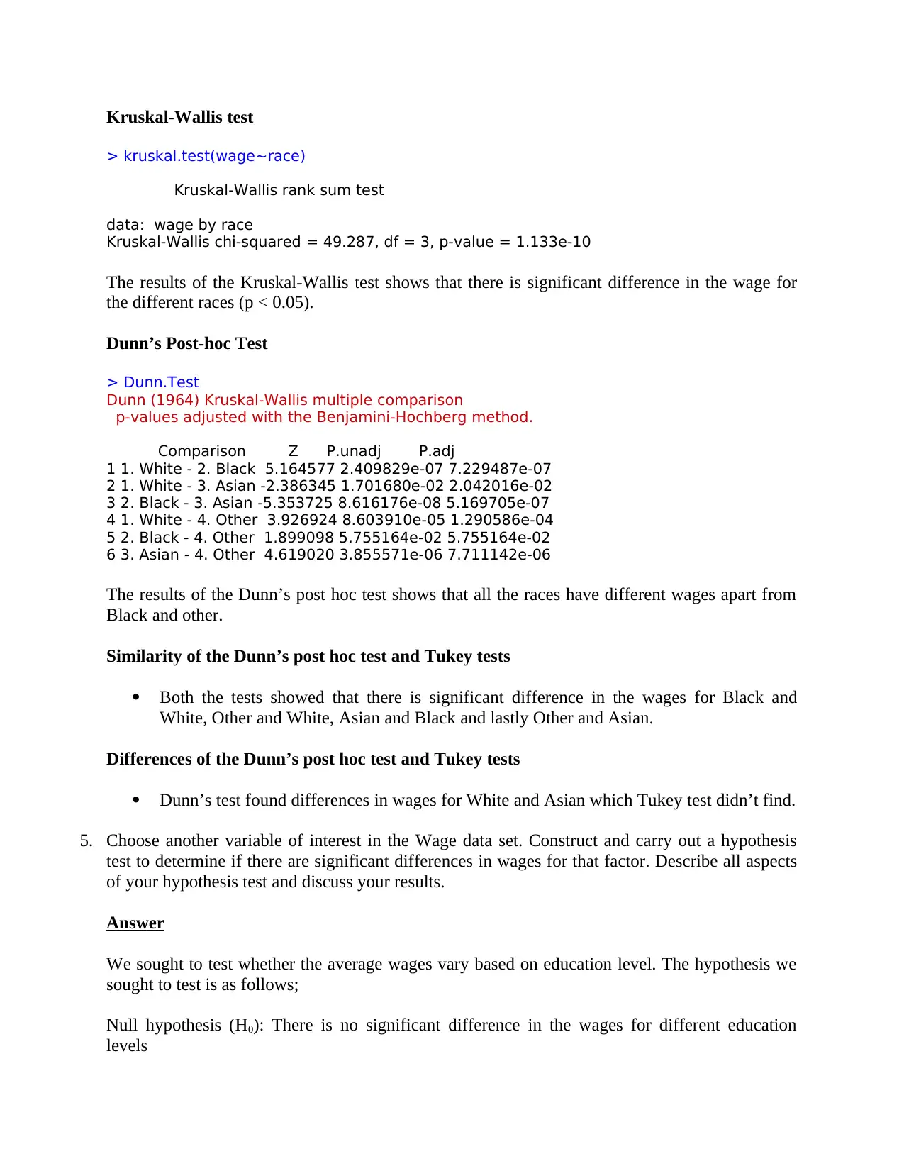
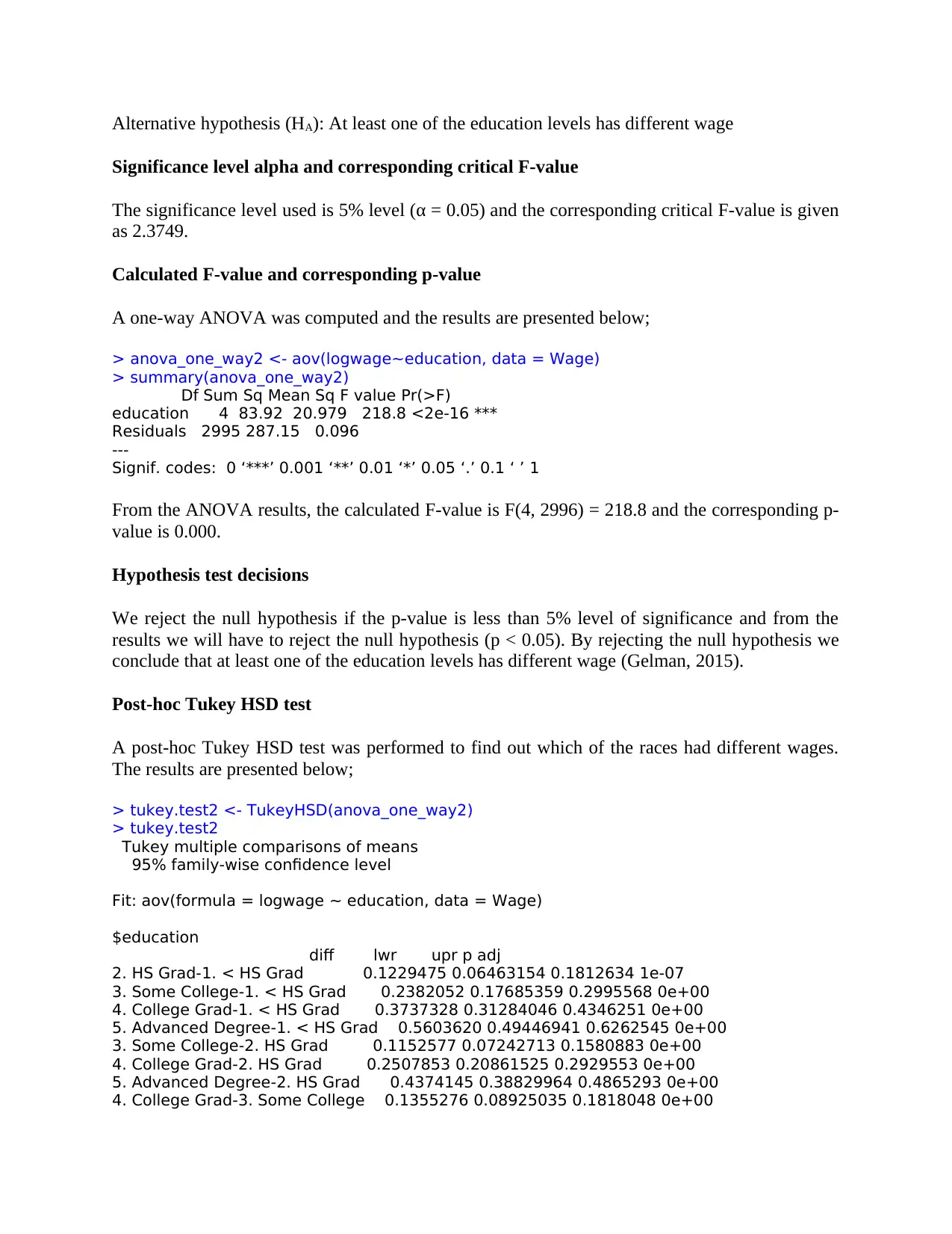
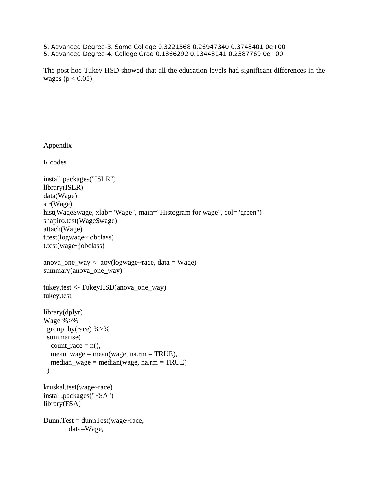
This assignment analyzes the Wage dataset using various statistical techniques to perform hypothesis testing. The student assesses the normality of the wage variable, finding it non-normal and suggesting a transformation. The assignment then uses an independent t-test to compare wages between the information and industrial sectors, rejecting the null hypothesis and concluding a significant wage difference. A one-way ANOVA is employed to determine wage differences across races, leading to the rejection of the null hypothesis and a post-hoc Tukey HSD test identifies specific racial wage disparities. The student also explores non-parametric methods like the Kruskal-Wallis test and Dunn's post-hoc test for comparison. Finally, the student conducts another hypothesis test, using a one-way ANOVA to analyze wage differences based on education levels, rejecting the null hypothesis and using a post-hoc Tukey HSD to determine which education levels have significant wage differences. The assignment includes R code and references.

Hypothesis Testing
Student Name:
Instructor Name:
Course Number:
23rd March 2020

1. Analysis techniques such as t-test or one-way ANOVA assume that the data being compared
comes from normal distributions. Assess the normality of the wage variable in the Wage data set.
Is a normal assumption appropriate? If not, what normal transformation can be applied? In the
comparisons to assess significant differences, you should use the transformed values.
Answer
We assess the normality of the wage variable in the Wage data set using a histogram as shown
below;
From the above histogram, it is evident that the wage variable is not normally distributed but is
rather skewed to the right (longer tail to the right).
We confirm this using Shapiro-Wilk test where the results are presented below;
> shapiro.test(Wage$wage)
Shapiro-Wilk normality test
data: Wage$wage
W = 0.87957, p-value < 2.2e-16
The above results further confirm that the variable wage is does not follow a normal distribution
(p < 0.05).
2. Use an independent t-test to determine whether or not there is a significant difference in wages
for the information and industrial sectors using the variable jobclass.
Answer

Null and alternative hypotheses
In this section we sought to test the following hypothesis;
Null hypothesis (H0): There is no significant difference in the wages for the information and
industrial sectors.
Alternative hypothesis (HA): There is significant difference in the wages for the information and
industrial sectors.
Significance level alpha and corresponding critical t-value
The significance level used is 5% level (α = 0.05) and the corresponding critical t-value is given
as 1.961.
Calculated t-value and corresponding p-value
An independent t-test was computed and the results are presented below;
> t.test(logwage~jobclass)
Welch Two Sample t-test
data: logwage by jobclass
t = -11.468, df = 2948.3, p-value < 2.2e-16
alternative hypothesis: true difference in means is not equal to 0
95 percent confidence interval:
-0.1692574 -0.1198298
sample estimates:
mean in group 1. Industrial mean in group 2. Information
4.583753 4.728297
From the t-test results, the calculated t-value is t = -11.468 and the corresponding p-value is
0.000 (Fay & Proschan, 2014).
Hypothesis test decisions
We reject the null hypothesis if the p-value is less than 5% level of significance and from the
results we will have to reject the null hypothesis (p < 0.05).
Statement as to whether that alternative hypothesis is true
Rejecting the null hypothesis implies that the alternative hypothesis is true.
Description of what the hypothesis means

By rejecting the null hypothesis and accepting the alternative we conclude that there is
significant difference in the wages for the information and industrial sectors. The average
difference in wages for the two sectors is 17.27.
3. Use a one-way ANOVA to determine whether or not there is a significant difference in wages for
different races using the variable race. Include the following:
Answer
Null and alternative hypotheses
In this section we sought to test the following hypothesis;
Null hypothesis (H0): There is no significant difference in the wages for different races
Alternative hypothesis (HA): At least one of the races has different wage
Significance level alpha and corresponding critical F-value
The significance level used is 5% level (α = 0.05) and the corresponding critical F-value is given
as 2.6079 (Anscombe, 2018).
Calculated F-value and corresponding p-value
A one-way ANOVA was computed and the results are presented below;
> anova_one_way <- aov(logwage~race, data = Wage)
> summary(anova_one_way)
Df Sum Sq Mean Sq F value Pr(>F)
race 3 4.5 1.5129 12.37 4.88e-08 ***
Residuals 2996 366.5 0.1223
---
Signif. codes: 0 ‘***’ 0.001 ‘**’ 0.01 ‘*’ 0.05 ‘.’ 0.1 ‘ ’ 1
From the ANOVA results, the calculated F-value is F(3, 2996) = 12.37 and the corresponding p-
value is 0.000.
Hypothesis test decisions
We reject the null hypothesis if the p-value is less than 5% level of significance and from the
results we will have to reject the null hypothesis (p < 0.05). By rejecting the null hypothesis we
conclude that at least one of the races had a different wage.
Post-hoc Tukey HSD test
A post-hoc Tukey HSD test was performed to find out which of the races had different wages.
The results are presented below;

> tukey.test <- TukeyHSD(anova_one_way)
> tukey.test
Tukey multiple comparisons of means
95% family-wise confidence level
Fit: aov(formula = logwage ~ race, data = Wage)
$race
diff lwr upr p adj
2. Black-1. White -0.09089699 -0.14643760 -0.03535638 0.0001564
3. Asian-1. White 0.05868398 -0.00899415 0.12636211 0.1156882
4. Other-1. White -0.21081288 -0.35971821 -0.06190754 0.0015840
3. Asian-2. Black 0.14958097 0.06583608 0.23332585 0.0000272
4. Other-2. Black -0.11991589 -0.27677785 0.03694608 0.2015539
4. Other-3. Asian -0.26949686 -0.43105565 -0.10793806 0.0001095
The races that had significant differences in wages are;
 Black and White
 Other and White
 Asian and Black
 Other and Asian
Mean and median wages for each of the races
The mean and median wages for each of the races is presented below;
# A tibble: 4 x 4
race count_race mean_wage median_wage
<fct> <int> <dbl> <dbl>
1 1. White 2480 113. 106.
2 2. Black 293 102. 94.1
3 3. Asian 190 120. 115.
4 4. Other 37 90.0 81.3
Mean wage for the White is 113.0 while for the Asian it was 120.0 and 102.0 and 90.0 for the
Black and other respectively.
Discussing results
Taken together, the results shows that workers of Asian origin have on average highest average
wage (M = 120.0) followed by the workers of White origin (M = 113.0). Black workers are the
third in terms of the wages (M = 102.0) while the other races are the least paid (M = 90.0)
4. The log (Wage) transformation allowed you to meet the normal assumptions for ANOVA,
however, this is not always possible. Consider differences in Wage by race using non-parametric
techniques.
Answer

Kruskal-Wallis test
> kruskal.test(wage~race)
Kruskal-Wallis rank sum test
data: wage by race
Kruskal-Wallis chi-squared = 49.287, df = 3, p-value = 1.133e-10
The results of the Kruskal-Wallis test shows that there is significant difference in the wage for
the different races (p < 0.05).
Dunn’s Post-hoc Test
> Dunn.Test
Dunn (1964) Kruskal-Wallis multiple comparison
p-values adjusted with the Benjamini-Hochberg method.
Comparison Z P.unadj P.adj
1 1. White - 2. Black 5.164577 2.409829e-07 7.229487e-07
2 1. White - 3. Asian -2.386345 1.701680e-02 2.042016e-02
3 2. Black - 3. Asian -5.353725 8.616176e-08 5.169705e-07
4 1. White - 4. Other 3.926924 8.603910e-05 1.290586e-04
5 2. Black - 4. Other 1.899098 5.755164e-02 5.755164e-02
6 3. Asian - 4. Other 4.619020 3.855571e-06 7.711142e-06
The results of the Dunn’s post hoc test shows that all the races have different wages apart from
Black and other.
Similarity of the Dunn’s post hoc test and Tukey tests
 Both the tests showed that there is significant difference in the wages for Black and
White, Other and White, Asian and Black and lastly Other and Asian.
Differences of the Dunn’s post hoc test and Tukey tests
 Dunn’s test found differences in wages for White and Asian which Tukey test didn’t find.
5. Choose another variable of interest in the Wage data set. Construct and carry out a hypothesis
test to determine if there are significant differences in wages for that factor. Describe all aspects
of your hypothesis test and discuss your results.
Answer
We sought to test whether the average wages vary based on education level. The hypothesis we
sought to test is as follows;
Null hypothesis (H0): There is no significant difference in the wages for different education
levels

Alternative hypothesis (HA): At least one of the education levels has different wage
Significance level alpha and corresponding critical F-value
The significance level used is 5% level (α = 0.05) and the corresponding critical F-value is given
as 2.3749.
Calculated F-value and corresponding p-value
A one-way ANOVA was computed and the results are presented below;
> anova_one_way2 <- aov(logwage~education, data = Wage)
> summary(anova_one_way2)
Df Sum Sq Mean Sq F value Pr(>F)
education 4 83.92 20.979 218.8 <2e-16 ***
Residuals 2995 287.15 0.096
---
Signif. codes: 0 ‘***’ 0.001 ‘**’ 0.01 ‘*’ 0.05 ‘.’ 0.1 ‘ ’ 1
From the ANOVA results, the calculated F-value is F(4, 2996) = 218.8 and the corresponding p-
value is 0.000.
Hypothesis test decisions
We reject the null hypothesis if the p-value is less than 5% level of significance and from the
results we will have to reject the null hypothesis (p < 0.05). By rejecting the null hypothesis we
conclude that at least one of the education levels has different wage (Gelman, 2015).
Post-hoc Tukey HSD test
A post-hoc Tukey HSD test was performed to find out which of the races had different wages.
The results are presented below;
> tukey.test2 <- TukeyHSD(anova_one_way2)
> tukey.test2
Tukey multiple comparisons of means
95% family-wise confidence level
Fit: aov(formula = logwage ~ education, data = Wage)
$education
diff lwr upr p adj
2. HS Grad-1. < HS Grad 0.1229475 0.06463154 0.1812634 1e-07
3. Some College-1. < HS Grad 0.2382052 0.17685359 0.2995568 0e+00
4. College Grad-1. < HS Grad 0.3737328 0.31284046 0.4346251 0e+00
5. Advanced Degree-1. < HS Grad 0.5603620 0.49446941 0.6262545 0e+00
3. Some College-2. HS Grad 0.1152577 0.07242713 0.1580883 0e+00
4. College Grad-2. HS Grad 0.2507853 0.20861525 0.2929553 0e+00
5. Advanced Degree-2. HS Grad 0.4374145 0.38829964 0.4865293 0e+00
4. College Grad-3. Some College 0.1355276 0.08925035 0.1818048 0e+00

5. Advanced Degree-3. Some College 0.3221568 0.26947340 0.3748401 0e+00
5. Advanced Degree-4. College Grad 0.1866292 0.13448141 0.2387769 0e+00
The post hoc Tukey HSD showed that all the education levels had significant differences in the
wages (p < 0.05).
Appendix
R codes
install.packages("ISLR")
library(ISLR)
data(Wage)
str(Wage)
hist(Wage$wage, xlab="Wage", main="Histogram for wage", col="green")
shapiro.test(Wage$wage)
attach(Wage)
t.test(logwage~jobclass)
t.test(wage~jobclass)
anova_one_way <- aov(logwage~race, data = Wage)
summary(anova_one_way)
tukey.test <- TukeyHSD(anova_one_way)
tukey.test
library(dplyr)
Wage %>%
group_by(race) %>%
summarise(
count_race = n(),
mean_wage = mean(wage, na.rm = TRUE),
median_wage = median(wage, na.rm = TRUE)
)
kruskal.test(wage~race)
install.packages("FSA")
library(FSA)
Dunn.Test = dunnTest(wage~race,
data=Wage,

method="bh")
Dunn.Test
anova_one_way2 <- aov(logwage~education, data = Wage)
summary(anova_one_way2)
tukey.test2 <- TukeyHSD(anova_one_way2)
tukey.test2
References
Anscombe, F. J. (2018). The Validity of Comparative Experiments. Journal of the Royal
Statistical Society, 111(3), 181–211.
Fay, M. P., & Proschan, M. A. (2014). Wilcoxon–Mann–Whitney or t-test? On assumptions for
hypothesis tests and multiple interpretations of decision rules. Statistics Surveys, 4, 1–39.
Gelman, A. (2015). Analysis of variance? Why it is more important than ever. The Annals of
Statistics, 33, 1–53.