NIT3171: ICT Business Analysis and Data Visualization Report

This report presents a comprehensive analysis of the Boston Housing Dataset, focusing on data visualization and business analytics techniques. The analysis begins with an introduction to the dataset, describing its variables and characteristics. Task 1 involves visualizing categorical and quantitative variables, including histograms, bar graphs, and pie charts to understand the distribution and properties of the data. Task 2 explores the relationships between variables, such as the correlation between house condition and sales price, garage quality and sales price, and the impact of lot size and building age on sales prices, utilizing scatter plots and other visualizations. Task 3 focuses on building a regression model to predict sales prices, identifying significant variables like living area and lot area, and assessing the model's performance. The conclusion highlights the potential for further analysis and the importance of data-driven decision-making in business. The report provides a detailed overview of the dataset and the factors influencing house prices and provides insights for business decisions.

Running head: ICT BUS ANANLYTICS AND DATA VISUALATION
ICT BUS ANANLYTICS AND DATA VISUALATION
Name of the University
Name of the Student
Author’s Note

2ICT BUS ANANLYTICS AND DATA VISUALATION
Table of Contents
Introduction:...............................................................................................................................2
Task 1:........................................................................................................................................2
Task 2:........................................................................................................................................7
Task 3:......................................................................................................................................12
Conclusion:..............................................................................................................................12
References:...............................................................................................................................13

3ICT BUS ANANLYTICS AND DATA VISUALATION
Introduction:
The Boston Housing Dataset consists of information about houses in Boston and has
1461 values. There are 24 nominal, 25 ordinal, 15 discrete and 20 continuous variables out of
the total 83 variables describing the various attributes of the variables. Several of the
variables have missing values and they need to be dealt with standard techniques before
working with them for predicting any variable.
Task 1:
Visualization and Descriptive Statistics of the variables:
Some of the categorical variables in the dataset are described below:
MSSubClass: Identifies the type of dwelling involved in the sale.
MSZoning: Identifies the general zoning classification of the sale.
Street: Type of road access to property.
Alley: Type of alley access to property
LotShape: General shape of property
LandContour: Flatness of the property
Utilities: Type of utilities available
LotConfig: Lot configuration
LandSlope: Slope of property
Neighborhood: Physical locations within Ames city limits
Condition1: Proximity to various conditions
Condition2: Proximity to various conditions (if more than one is present)
Garageb Qual: Garage quality further subdivided as:

4ICT BUS ANANLYTICS AND DATA VISUALATION
Ex Excellent
Gd Good
TA Typical/Average
Fa Fair
Po Poor
NA No Garage
Sale Condition: Condition of sale further divided as:
Normal: Normal Sale
Abnorml: Abnormal Sale - trade, foreclosure, short sale
AdjLand: Adjoining Land Purchase
Alloca: Allocation - two linked properties with separate deeds, typically condo with a garage unit
Family: Sale between family members
Partial: Home was not completed when last assessed (associated with New Homes)
GarageQual: Garage quality
Ex Excellent
Gd Good
TA Typical/Average
Fa Fair
Po Poor
NA No Garage
BldgType: Type of dwelling.
HouseStyle: Style of dwelling
Some of the quantitative variable are:
LotFrontage: Linear feet of street connected to property.
LotArea: Lot size in square feet.
GrLivArea: Above grade (ground) living area square feet
OverallQual: Rates the overall material and finish of the house
OverallCond: Rates the overall condition of the house
YearBuilt: Original construction date
As there are numerous variables in the dataset, a proper description is written in the excel file
attached along with the analysis done here.

5ICT BUS ANANLYTICS AND DATA VISUALATION
After familiarizing with the variables involved in the dataset, a basic exploratory data
analysis was done to see the properties of the variables.
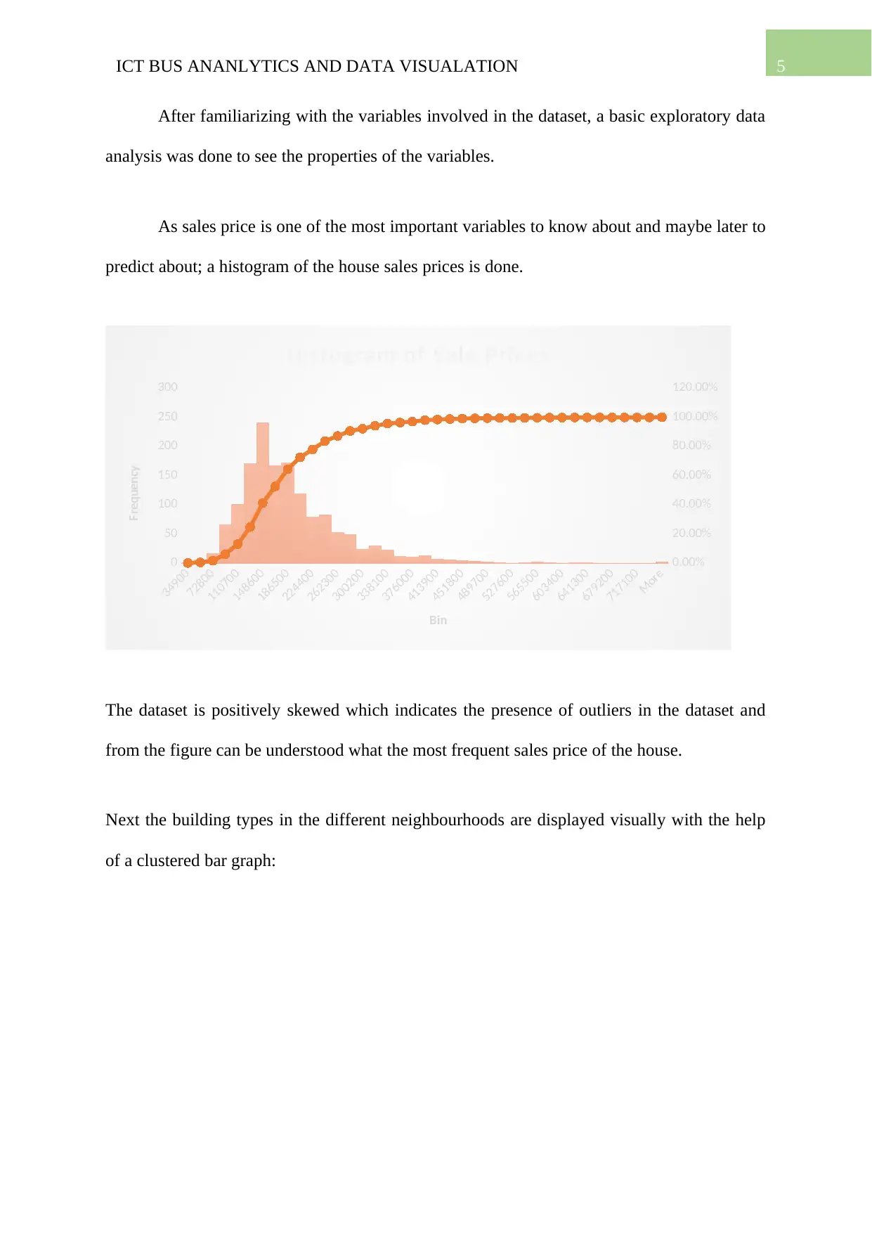
As sales price is one of the most important variables to know about and maybe later to
predict about; a histogram of the house sales prices is done.
34900
72800
110700
148600
186500
224400
262300
300200
338100
376000
413900
451800
489700
527600
565500
603400
641300
679200
717100
More
0
50
100
150
200
250
300
0.00%
20.00%
40.00%
60.00%
80.00%
100.00%
120.00%
Histogram of Sale Prices
Bin
Frequency
The dataset is positively skewed which indicates the presence of outliers in the dataset and
from the figure can be understood what the most frequent sales price of the house.
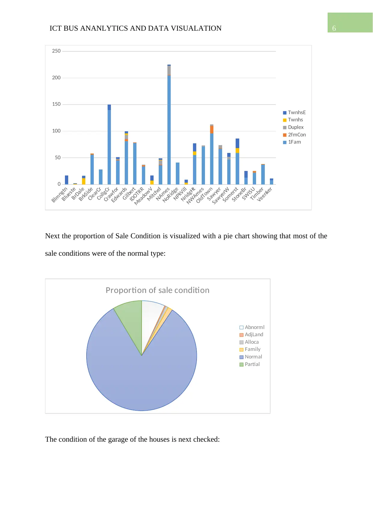
Next the building types in the different neighbourhoods are displayed visually with the help
of a clustered bar graph:

6ICT BUS ANANLYTICS AND DATA VISUALATION
Blmngtn
Blueste
BrDale
BrkSide
ClearCr
CollgCr
Crawfor
Edwards
Gilbert
IDOTRR
MeadowV
Mitchel
NAmes
NoRidge
NPkVill
NridgHt
NWAmes
OldTown
Sawyer
SawyerW
Somerst
StoneBr
SWISU
Timber
Veenker
0
50
100
150
200
250
TwnhsE
Twnhs
Duplex
2fmCon
1Fam
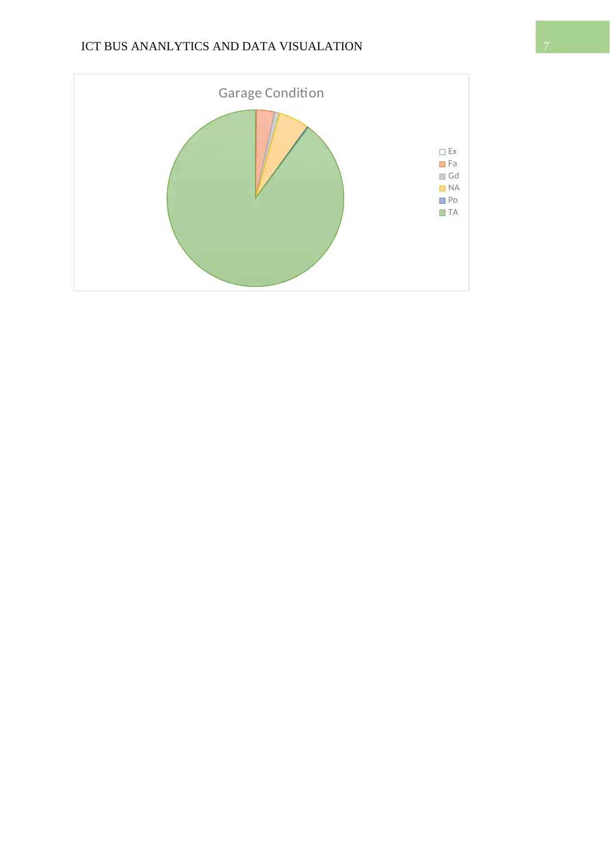
Next the proportion of Sale Condition is visualized with a pie chart showing that most of the
sale conditions were of the normal type:
Proportion of sale condition
Abnorml
AdjLand
Alloca
Family
Normal
Partial
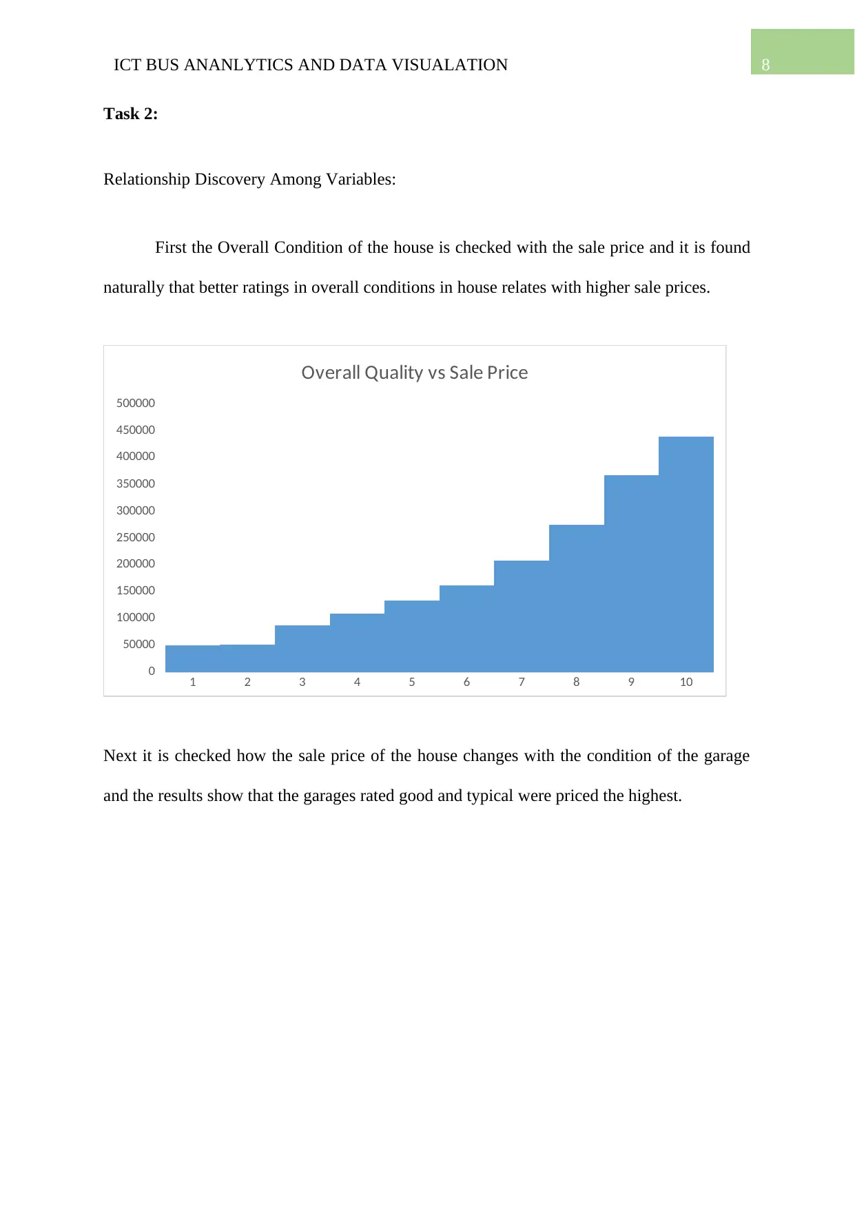
The condition of the garage of the houses is next checked:

7ICT BUS ANANLYTICS AND DATA VISUALATION
Garage Condition
Ex
Fa
Gd
NA
Po
TA

8ICT BUS ANANLYTICS AND DATA VISUALATION
Task 2:
Relationship Discovery Among Variables:
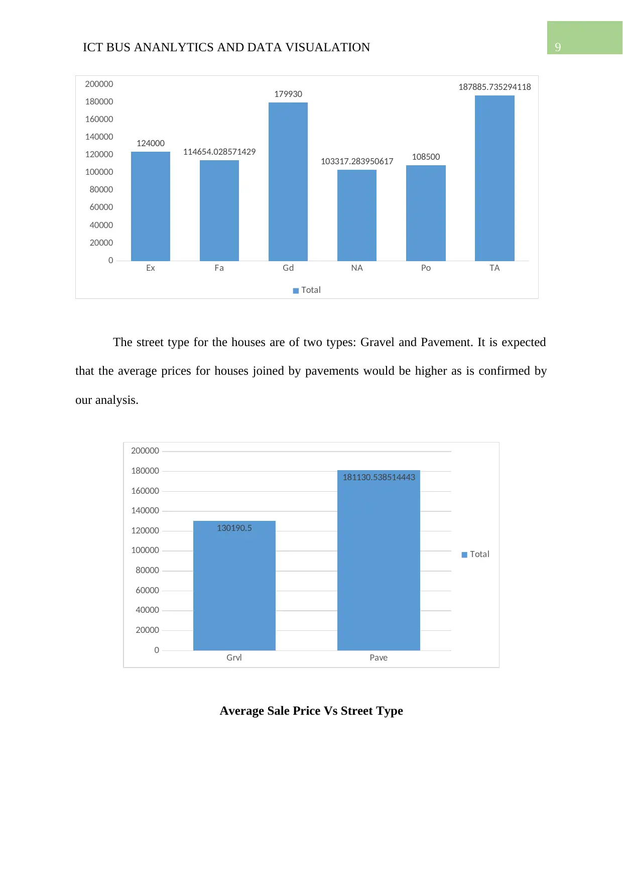
First the Overall Condition of the house is checked with the sale price and it is found
naturally that better ratings in overall conditions in house relates with higher sale prices.
1 2 3 4 5 6 7 8 9 10
0
50000
100000
150000
200000
250000
300000
350000
400000
450000
500000
Overall Quality vs Sale Price
Next it is checked how the sale price of the house changes with the condition of the garage
and the results show that the garages rated good and typical were priced the highest.

9ICT BUS ANANLYTICS AND DATA VISUALATION
Ex Fa Gd NA Po TA
0
20000
40000
60000
80000
100000
120000
140000
160000
180000
200000
124000 114654.028571429
179930
103317.283950617 108500
187885.735294118
Total
The street type for the houses are of two types: Gravel and Pavement. It is expected
that the average prices for houses joined by pavements would be higher as is confirmed by
our analysis.
Grvl Pave
0
20000
40000
60000
80000
100000
120000
140000
160000
180000
200000
130190.5
181130.538514443
Total
Average Sale Price Vs Street Type

10ICT BUS ANANLYTICS AND DATA VISUALATION
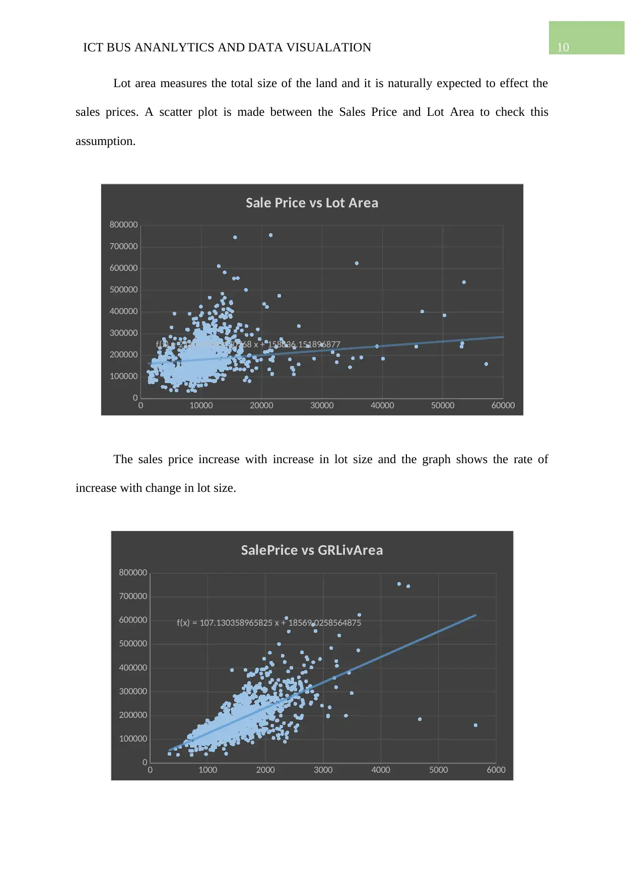
Lot area measures the total size of the land and it is naturally expected to effect the
sales prices. A scatter plot is made between the Sales Price and Lot Area to check this
assumption.
0 10000 20000 30000 40000 50000 60000
0
100000
200000
300000
400000
500000
600000
700000
800000
f(x) = 2.09997195170768 x + 158836.151896877
Sale Price vs Lot Area
The sales price increase with increase in lot size and the graph shows the rate of
increase with change in lot size.
0 1000 2000 3000 4000 5000 6000
0
100000
200000
300000
400000
500000
600000
700000
800000
f(x) = 107.130358965825 x + 18569.0258564875
SalePrice vs GRLivArea

11ICT BUS ANANLYTICS AND DATA VISUALATION
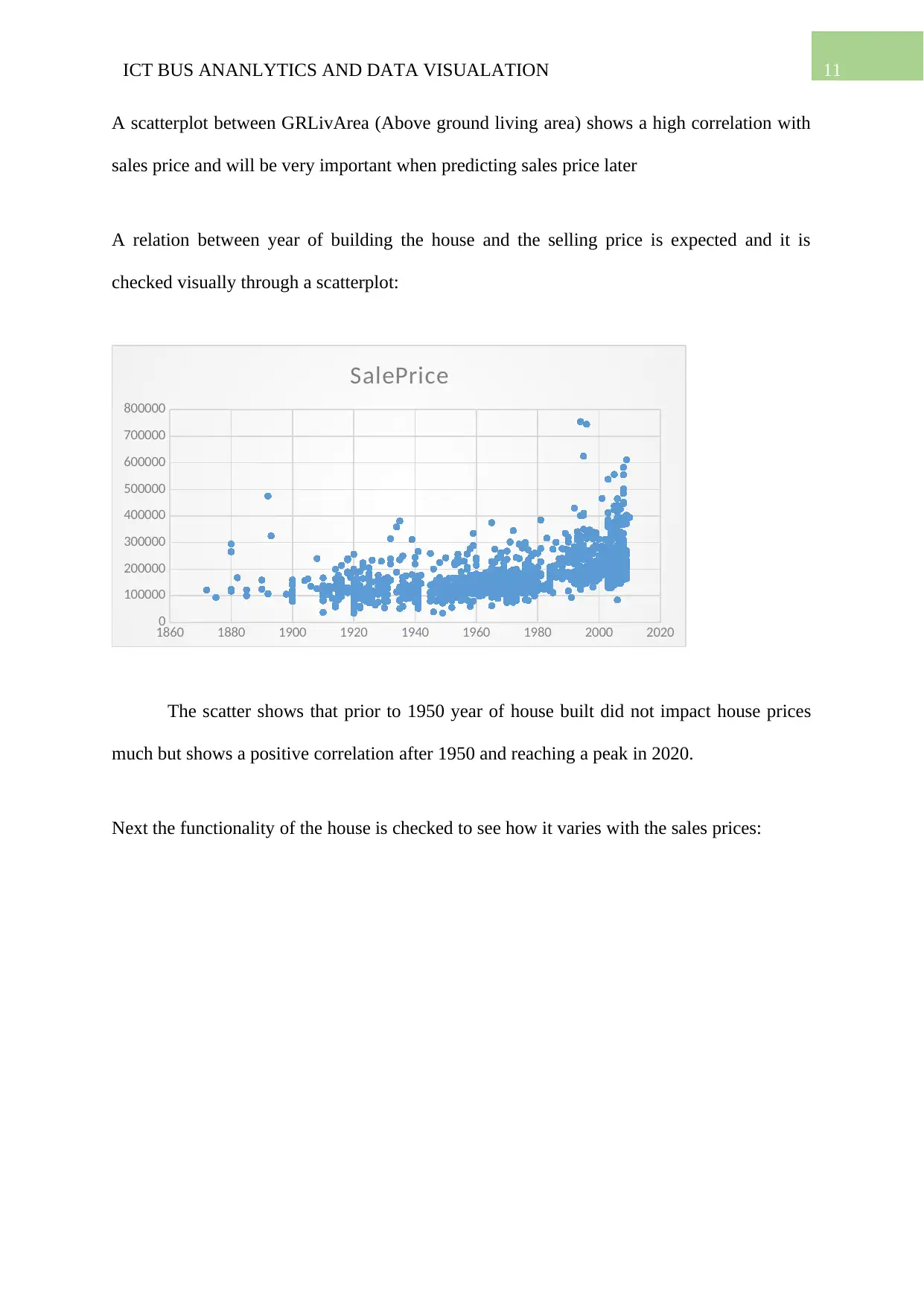
A scatterplot between GRLivArea (Above ground living area) shows a high correlation with
sales price and will be very important when predicting sales price later
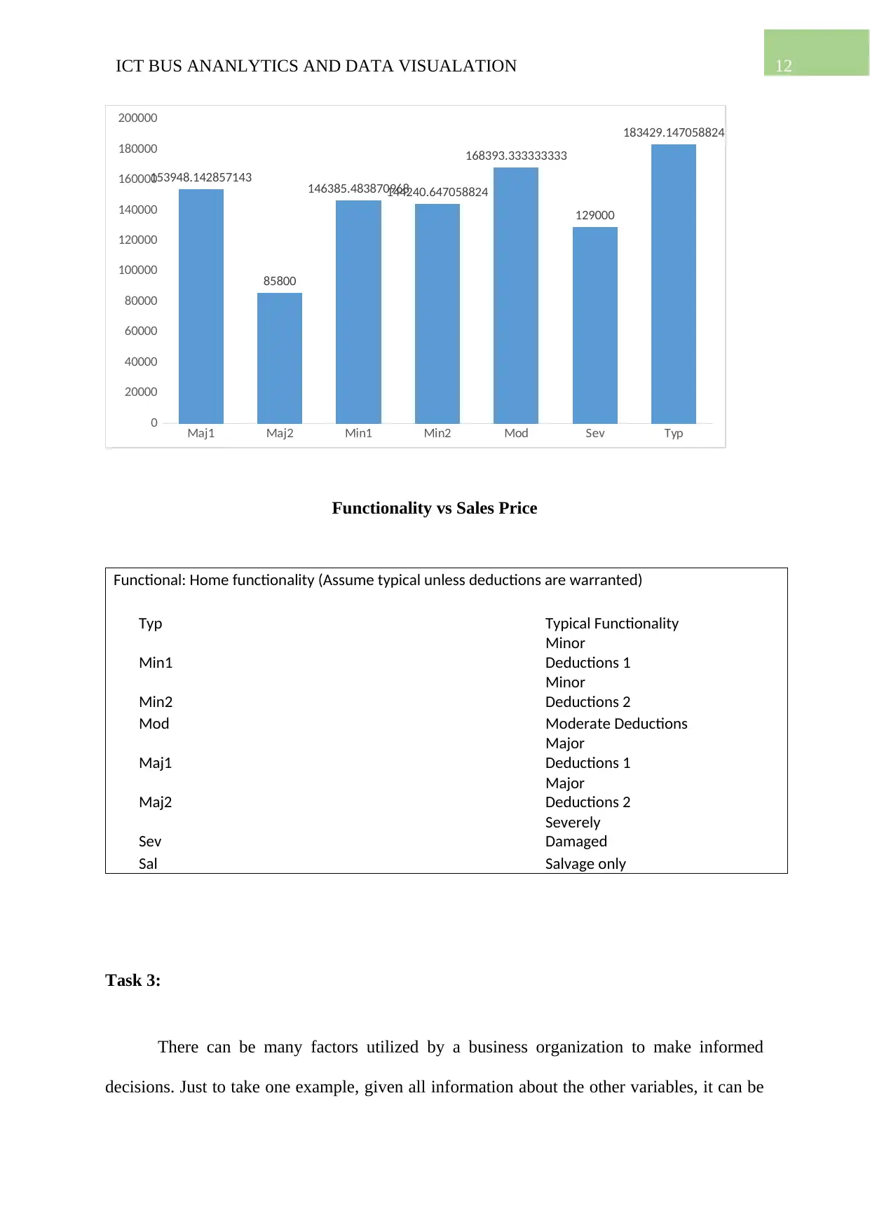
A relation between year of building the house and the selling price is expected and it is
checked visually through a scatterplot:
1860 1880 1900 1920 1940 1960 1980 2000 2020
0
100000
200000
300000
400000
500000
600000
700000
800000
SalePrice
The scatter shows that prior to 1950 year of house built did not impact house prices
much but shows a positive correlation after 1950 and reaching a peak in 2020.
Next the functionality of the house is checked to see how it varies with the sales prices:

12ICT BUS ANANLYTICS AND DATA VISUALATION
Maj1 Maj2 Min1 Min2 Mod Sev Typ
0
20000
40000
60000
80000
100000
120000
140000
160000
180000
200000
153948.142857143
85800
146385.483870968144240.647058824
168393.333333333
129000
183429.147058824
Functionality vs Sales Price
Functional: Home functionality (Assume typical unless deductions are warranted)
Typ Typical Functionality
Min1
Minor
Deductions 1
Min2
Minor
Deductions 2
Mod Moderate Deductions
Maj1
Major
Deductions 1
Maj2
Major
Deductions 2
Sev
Severely
Damaged
Sal Salvage only
Task 3:
There can be many factors utilized by a business organization to make informed
decisions. Just to take one example, given all information about the other variables, it can be

13ICT BUS ANANLYTICS AND DATA VISUALATION
predicted with some accuracy the selling price of a house. As it has been seen during the
exploratory data analysis some of the variables like GrLiv Area and Lot Area had positive
correlation with Sale Price it would be natural to gather the relevant variables and run a
regression to check how well the model works.
The regression run on excel show that the R squared value of the model at 0.68 thus
indicating that 68% of the variability of the Sales Price can be explained by the variability of
the dependent variables. However by interpreting the t stats and corresponding p values of the
coeffecients it must be noted that only GrLivArea, Lot Area, Pool Area, Screen Porch,
Enclosed Porch, WoodDeckSF, contribute significantly to the model.
Conclusion:
After analysing the dataset it can be said with a rich dataset like this there are always
better recommendations that can be made. Other sophisticated algorithms such as decision
trees, random forest can be used to predict the accuracy of predictions. And most importantly
the data analysis will depend upon the type of business organization and the kind of
information they wish to extract from the data.

14ICT BUS ANANLYTICS AND DATA VISUALATION
References:
Keller, P.R., Keller, M.M., Markel, S., Mallinckrodt, A.J. and McKay, S., 2014. Visual cues:
practical data visualization. Computers in Physics, 8(3), pp.297-298.
Liu, Y., 2014. Big data and predictive business analytics. The Journal of Business
Forecasting, 33(4), p.40.