IE 332 Engineering Statistics II Project

This document outlines a group project for the Engineering Statistics II course (IE 332) at King Abdulaziz University. The project requires students to apply statistical methods using Minitab and Excel to analyze provided datasets and draw conclusions. It includes tasks such as frequency distribution, hypothesis testing, confidence intervals, and analysis of variance. Students are also required to collect their own data for one question. The project emphasizes teamwork, practical application of statistical concepts, and the use of statistical software. The final submission includes a report, Minitab files, meeting minutes, and photos of the group's work.

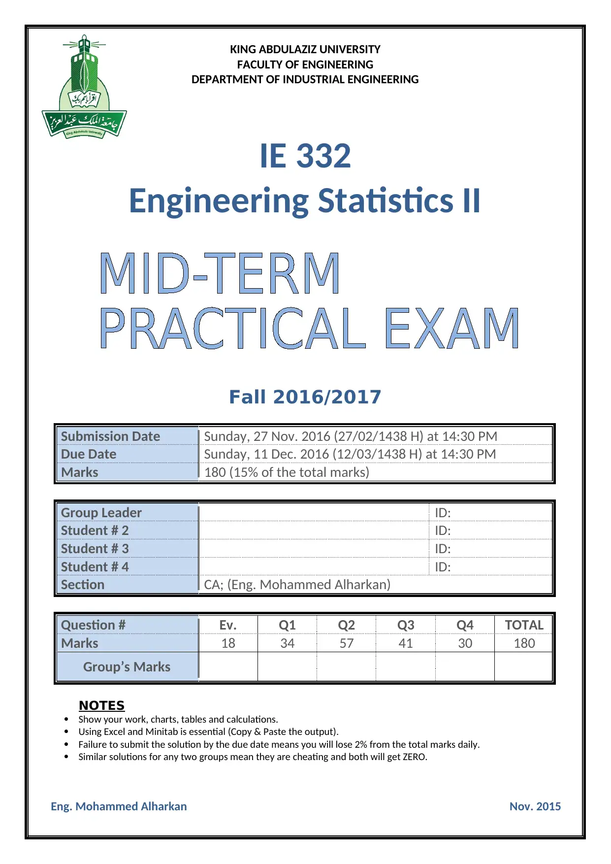
KING ABDULAZIZ UNIVERSITY
FACULTY OF ENGINEERING
DEPARTMENT OF INDUSTRIAL ENGINEERING
IE 332
Engineering Statistics II
Fall 2016/2017
Submission Date Sunday, 27 Nov. 2016 (27/02/1438 H) at 14:30 PM
Due Date Sunday, 11 Dec. 2016 (12/03/1438 H) at 14:30 PM
Marks 180 (15% of the total marks)
Group Leader ID:
Student # 2 ID:
Student # 3 ID:
Student # 4 ID:
Section CA; (Eng. Mohammed Alharkan)
Question # Ev. Q1 Q2 Q3 Q4 TOTAL
Marks 18 34 57 41 30 180
Group’s Marks
NOTES
 Show your work, charts, tables and calculations.
 Using Excel and Minitab is essential (Copy & Paste the output).
 Failure to submit the solution by the due date means you will lose 2% from the total marks daily.
 Similar solutions for any two groups mean they are cheating and both will get ZERO.
Eng. Mohammed Alharkan Nov. 2015

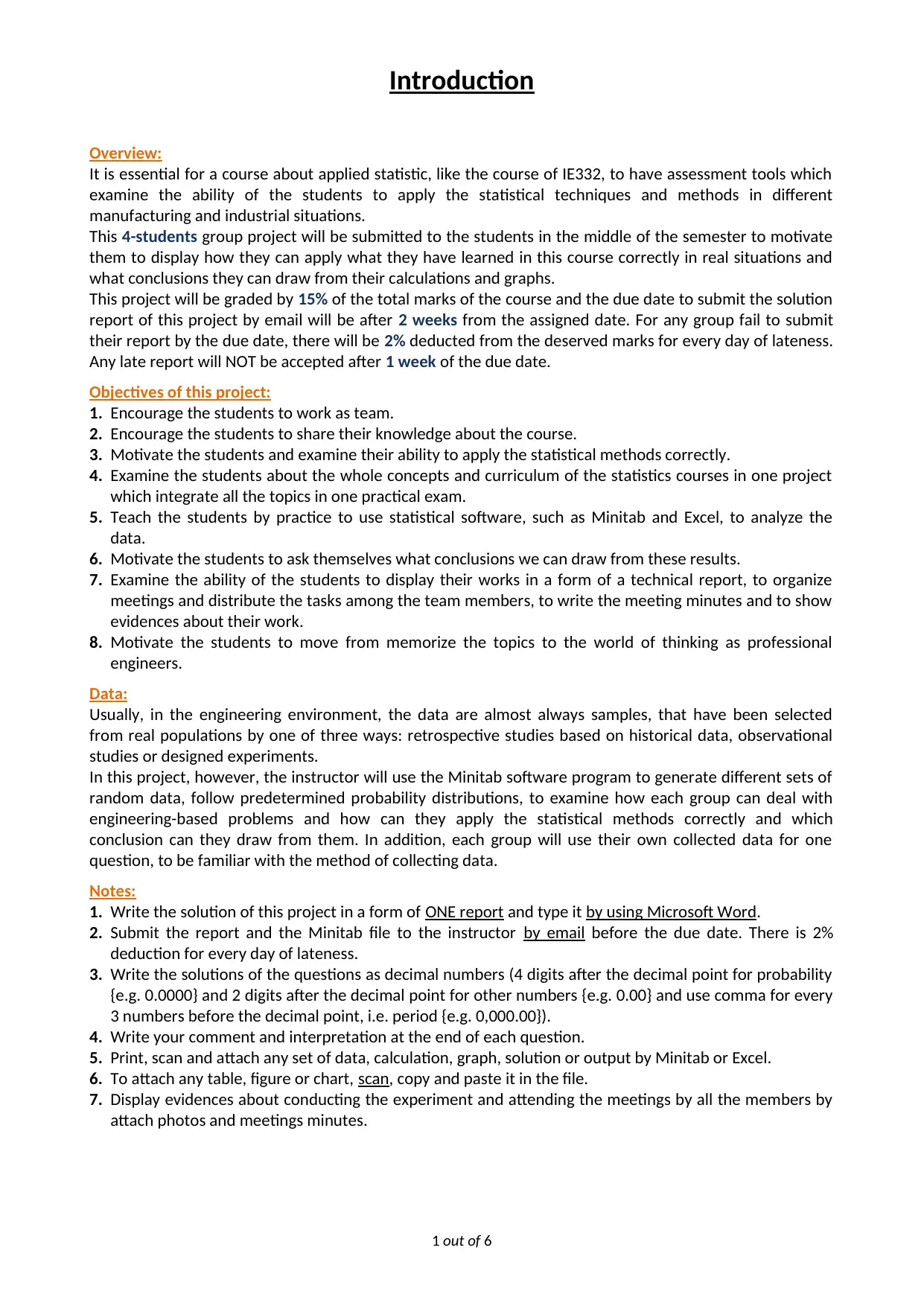
Introduction
Overview:
It is essential for a course about applied statistic, like the course of IE332, to have assessment tools which
examine the ability of the students to apply the statistical techniques and methods in different
manufacturing and industrial situations.
This 4-students group project will be submitted to the students in the middle of the semester to motivate
them to display how they can apply what they have learned in this course correctly in real situations and
what conclusions they can draw from their calculations and graphs.
This project will be graded by 15% of the total marks of the course and the due date to submit the solution
report of this project by email will be after 2 weeks from the assigned date. For any group fail to submit
their report by the due date, there will be 2% deducted from the deserved marks for every day of lateness.
Any late report will NOT be accepted after 1 week of the due date.
Objectives of this project:
1. Encourage the students to work as team.
2. Encourage the students to share their knowledge about the course.
3. Motivate the students and examine their ability to apply the statistical methods correctly.
4. Examine the students about the whole concepts and curriculum of the statistics courses in one project
which integrate all the topics in one practical exam.
5. Teach the students by practice to use statistical software, such as Minitab and Excel, to analyze the
data.
6. Motivate the students to ask themselves what conclusions we can draw from these results.
7. Examine the ability of the students to display their works in a form of a technical report, to organize
meetings and distribute the tasks among the team members, to write the meeting minutes and to show
evidences about their work.
8. Motivate the students to move from memorize the topics to the world of thinking as professional
engineers.
Data:
Usually, in the engineering environment, the data are almost always samples, that have been selected
from real populations by one of three ways: retrospective studies based on historical data, observational
studies or designed experiments.
In this project, however, the instructor will use the Minitab software program to generate different sets of
random data, follow predetermined probability distributions, to examine how each group can deal with
engineering-based problems and how can they apply the statistical methods correctly and which
conclusion can they draw from them. In addition, each group will use their own collected data for one
question, to be familiar with the method of collecting data.
Notes:
1. Write the solution of this project in a form of ONE report and type it by using Microsoft Word.
2. Submit the report and the Minitab file to the instructor by email before the due date. There is 2%
deduction for every day of lateness.
3. Write the solutions of the questions as decimal numbers (4 digits after the decimal point for probability
{e.g. 0.0000} and 2 digits after the decimal point for other numbers {e.g. 0.00} and use comma for every
3 numbers before the decimal point, i.e. period {e.g. 0,000.00}).
4. Write your comment and interpretation at the end of each question.
5. Print, scan and attach any set of data, calculation, graph, solution or output by Minitab or Excel.
6. To attach any table, figure or chart, scan, copy and paste it in the file.
7. Display evidences about conducting the experiment and attending the meetings by all the members by
attach photos and meetings minutes.
1 out of 6

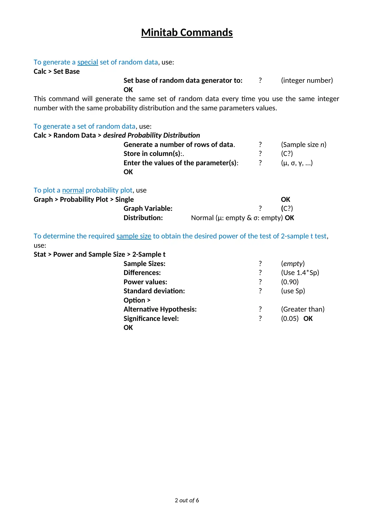
Minitab Commands
To generate a special set of random data, use:
Calc > Set Base
Set base of random data generator to: ? (integer number)
OK
This command will generate the same set of random data every time you use the same integer
number with the same probability distribution and the same parameters values.
To generate a set of random data, use:
Calc > Random Data > desired Probability Distribution
Generate a number of rows of data. ? (Sample size n)
Store in column(s):. ? (C?)
Enter the values of the parameter(s): ? (μ, σ, γ, …)
OK
To plot a normal probability plot, use
Graph > Probability Plot > Single OK
Graph Variable: ? (C?)
Distribution: Normal (μ: empty & σ: empty) OK
To determine the required sample size to obtain the desired power of the test of 2-sample t test,
use:
Stat > Power and Sample Size > 2-Sample t
Sample Sizes: ? (empty)
Differences: ? (Use 1.4*Sp)
Power values: ? (0.90)
Standard deviation: ? (use Sp)
Option >
Alternative Hypothesis: ? (Greater than)
Significance level: ? (0.05) OK
OK
2 out of 6

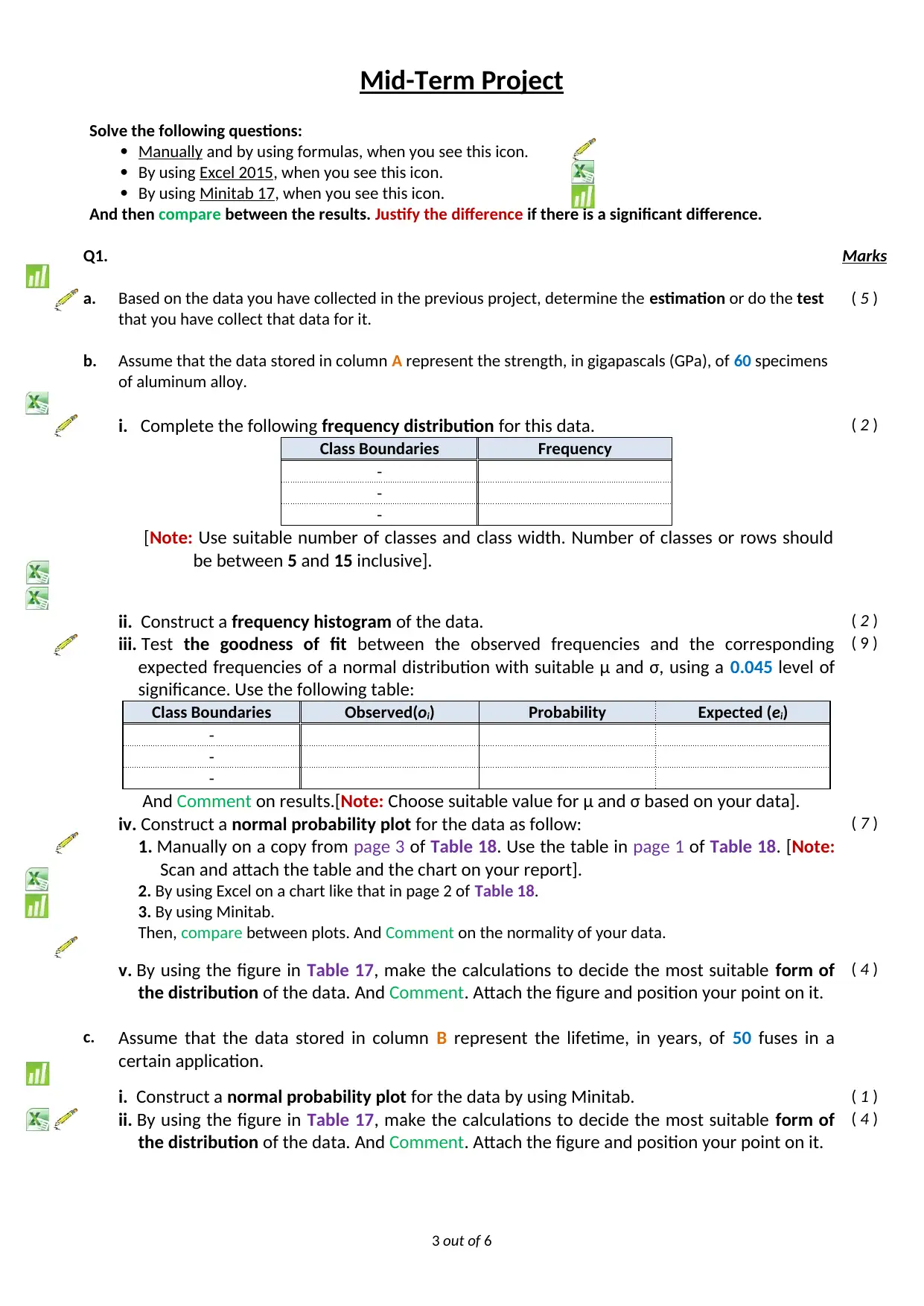
Mid-Term Project
Solve the following questions:
 Manually and by using formulas, when you see this icon.
 By using Excel 2015, when you see this icon.
 By using Minitab 17, when you see this icon.
And then compare between the results. Justify the difference if there is a significant difference.
Q1. Marks
a. Based on the data you have collected in the previous project, determine the estimation or do the test
that you have collect that data for it.
( 5 )
b. Assume that the data stored in column A represent the strength, in gigapascals (GPa), of 60 specimens
of aluminum alloy.
i. Complete the following frequency distribution for this data.
Class Boundaries Frequency
-
-
-
[Note: Use suitable number of classes and class width. Number of classes or rows should
be between 5 and 15 inclusive].
( 2 )
ii. Construct a frequency histogram of the data. ( 2 )
iii. Test the goodness of fit between the observed frequencies and the corresponding
expected frequencies of a normal distribution with suitable μ and σ, using a 0.045 level of
significance. Use the following table:
Class Boundaries Observed(oi) Probability Expected (ei)
-
-
-
And Comment on results.[Note: Choose suitable value for μ and σ based on your data].
( 9 )
iv. Construct a normal probability plot for the data as follow:
1. Manually on a copy from page 3 of Table 18. Use the table in page 1 of Table 18. [Note:
Scan and attach the table and the chart on your report].
2. By using Excel on a chart like that in page 2 of Table 18.
3. By using Minitab.
Then, compare between plots. And Comment on the normality of your data.
( 7 )
v. By using the figure in Table 17, make the calculations to decide the most suitable form of
the distribution of the data. And Comment. Attach the figure and position your point on it.
( 4 )
c. Assume that the data stored in column B represent the lifetime, in years, of 50 fuses in a
certain application.
i. Construct a normal probability plot for the data by using Minitab. ( 1 )
ii. By using the figure in Table 17, make the calculations to decide the most suitable form of
the distribution of the data. And Comment. Attach the figure and position your point on it.
( 4 )
3 out of 6

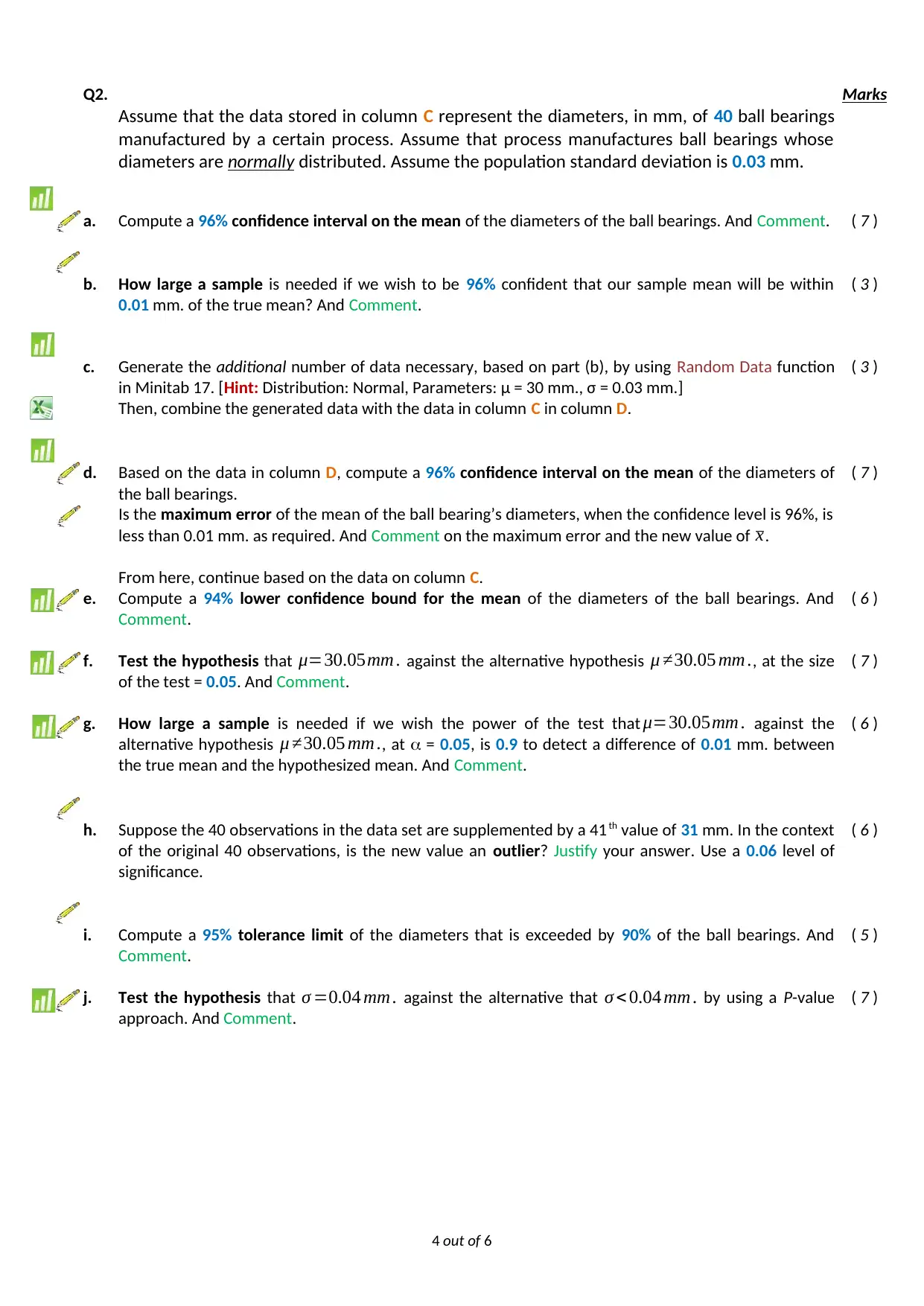
Q2. Marks
Assume that the data stored in column C represent the diameters, in mm, of 40 ball bearings
manufactured by a certain process. Assume that process manufactures ball bearings whose
diameters are normally distributed. Assume the population standard deviation is 0.03 mm.
a. Compute a 96% confidence interval on the mean of the diameters of the ball bearings. And Comment. ( 7 )
b. How large a sample is needed if we wish to be 96% confident that our sample mean will be within
0.01 mm. of the true mean? And Comment.
( 3 )
c. Generate the additional number of data necessary, based on part (b), by using Random Data function
in Minitab 17. [Hint: Distribution: Normal, Parameters: μ = 30 mm., σ = 0.03 mm.]
Then, combine the generated data with the data in column C in column D.
( 3 )
d. Based on the data in column D, compute a 96% confidence interval on the mean of the diameters of
the ball bearings.
Is the maximum error of the mean of the ball bearing’s diameters, when the confidence level is 96%, is
less than 0.01 mm. as required. And Comment on the maximum error and the new value of x.
( 7 )
From here, continue based on the data on column C.
e. Compute a 94% lower confidence bound for the mean of the diameters of the ball bearings. And
Comment.
( 6 )
f. Test the hypothesis that μ=30.05mm . against the alternative hypothesis μ ≠30.05 mm ., at the size
of the test = 0.05. And Comment.
( 7 )
g. How large a sample is needed if we wish the power of the test that μ=30.05mm . against the
alternative hypothesis μ ≠30.05 mm ., at  = 0.05, is 0.9 to detect a difference of 0.01 mm. between
the true mean and the hypothesized mean. And Comment.
( 6 )
h. Suppose the 40 observations in the data set are supplemented by a 41 th value of 31 mm. In the context
of the original 40 observations, is the new value an outlier? Justify your answer. Use a 0.06 level of
significance.
( 6 )
i. Compute a 95% tolerance limit of the diameters that is exceeded by 90% of the ball bearings. And
Comment.
( 5 )
j. Test the hypothesis that σ =0.04 mm . against the alternative that σ < 0.04 mm . by using a P-value
approach. And Comment.
( 7 )
4 out of 6

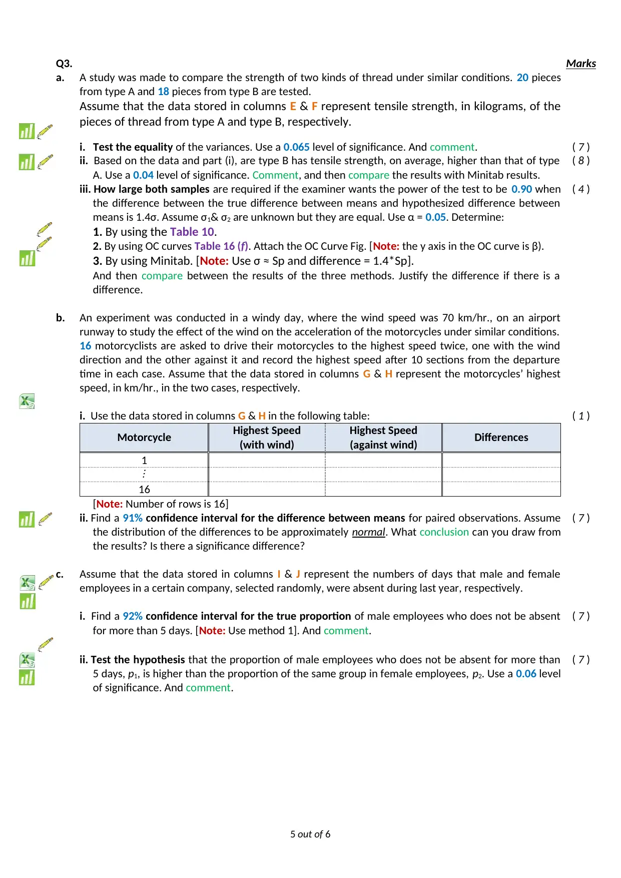
Q3. Marks
a. A study was made to compare the strength of two kinds of thread under similar conditions. 20 pieces
from type A and 18 pieces from type B are tested.
Assume that the data stored in columns E & F represent tensile strength, in kilograms, of the
pieces of thread from type A and type B, respectively.
i. Test the equality of the variances. Use a 0.065 level of significance. And comment. ( 7 )
ii. Based on the data and part (i), are type B has tensile strength, on average, higher than that of type
A. Use a 0.04 level of significance. Comment, and then compare the results with Minitab results.
( 8 )
iii. How large both samples are required if the examiner wants the power of the test to be 0.90 when
the difference between the true difference between means and hypothesized difference between
means is 1.4σ. Assume σ1& σ2 are unknown but they are equal. Use α = 0.05. Determine:
1. By using the Table 10.
2. By using OC curves Table 16 (f). Attach the OC Curve Fig. [Note: the y axis in the OC curve is β).
3. By using Minitab. [Note: Use σ ≈ Sp and difference = 1.4*Sp].
And then compare between the results of the three methods. Justify the difference if there is a
difference.
( 4 )
b. An experiment was conducted in a windy day, where the wind speed was 70 km/hr., on an airport
runway to study the effect of the wind on the acceleration of the motorcycles under similar conditions.
16 motorcyclists are asked to drive their motorcycles to the highest speed twice, one with the wind
direction and the other against it and record the highest speed after 10 sections from the departure
time in each case. Assume that the data stored in columns G & H represent the motorcycles’ highest
speed, in km/hr., in the two cases, respectively.
i. Use the data stored in columns G & H in the following table:
Motorcycle Highest Speed
(with wind)
Highest Speed
(against wind) Differences
1
⋮
16
[Note: Number of rows is 16]
( 1 )
ii. Find a 91% confidence interval for the difference between means for paired observations. Assume
the distribution of the differences to be approximately normal. What conclusion can you draw from
the results? Is there a significance difference?
( 7 )
c. Assume that the data stored in columns I & J represent the numbers of days that male and female
employees in a certain company, selected randomly, were absent during last year, respectively.
i. Find a 92% confidence interval for the true proportion of male employees who does not be absent
for more than 5 days. [Note: Use method 1]. And comment.
( 7 )
ii. Test the hypothesis that the proportion of male employees who does not be absent for more than
5 days, p1, is higher than the proportion of the same group in female employees, p2. Use a 0.06 level
of significance. And comment.
( 7 )
5 out of 6

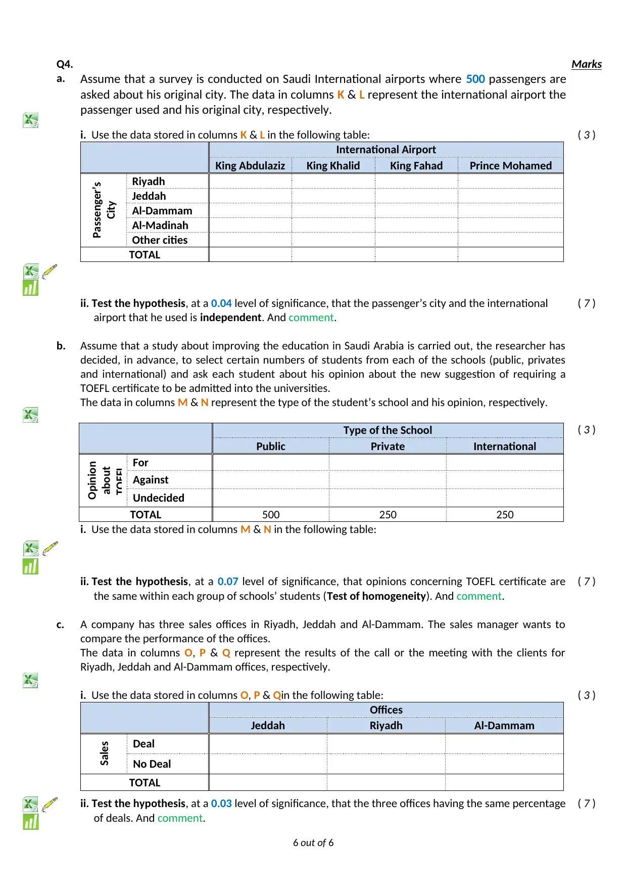
Q4. Marks
a. Assume that a survey is conducted on Saudi International airports where 500 passengers are
asked about his original city. The data in columns K & L represent the international airport the
passenger used and his original city, respectively.
i. Use the data stored in columns K & L in the following table:
International Airport
King Abdulaziz King Khalid King Fahad Prince Mohamed
Passenger’s
City
Riyadh
Jeddah
Al-Dammam
Al-Madinah
Other cities
TOTAL
( 3 )
ii. Test the hypothesis, at a 0.04 level of significance, that the passenger’s city and the international
airport that he used is independent. And comment.
( 7 )
b. Assume that a study about improving the education in Saudi Arabia is carried out, the researcher has
decided, in advance, to select certain numbers of students from each of the schools (public, privates
and international) and ask each student about his opinion about the new suggestion of requiring a
TOEFL certificate to be admitted into the universities.
The data in columns M & N represent the type of the student’s school and his opinion, respectively.
i. Use the data stored in columns M & N in the following table:
( 3 )
ii. Test the hypothesis, at a 0.07 level of significance, that opinions concerning TOEFL certificate are
the same within each group of schools’ students (Test of homogeneity). And comment.
( 7 )
c. A company has three sales offices in Riyadh, Jeddah and Al-Dammam. The sales manager wants to
compare the performance of the offices.
The data in columns O, P & Q represent the results of the call or the meeting with the clients for
Riyadh, Jeddah and Al-Dammam offices, respectively.
i. Use the data stored in columns O, P & Qin the following table:
Offices
Jeddah Riyadh Al-Dammam
Sales Deal
No Deal
TOTAL
( 3 )
ii. Test the hypothesis, at a 0.03 level of significance, that the three offices having the same percentage
of deals. And comment.
( 7 )
6 out of 6
Type of the School
Public Private International
Opinion
about
TOEFL For
Against
Undecided
TOTAL 500 250 250

Conclusion: ( 26 )
 Write about what you have learned in this project.
 Submit the meeting minutes at the end of the report with photos about the meeting and experiment.
GOOD LUCK
7 out of 6