Application of Implicit Functional Theorem (IFT) in Economics Analysis

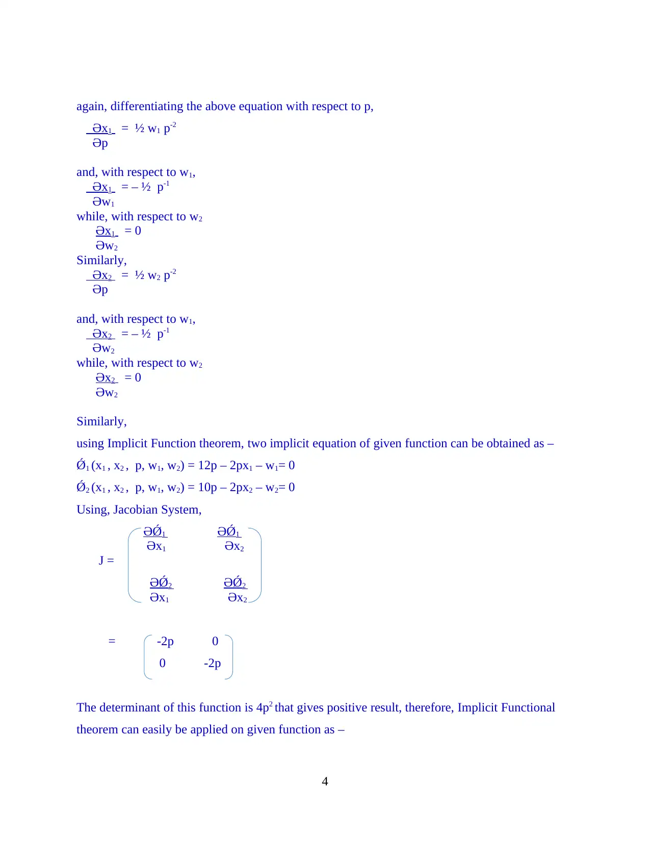
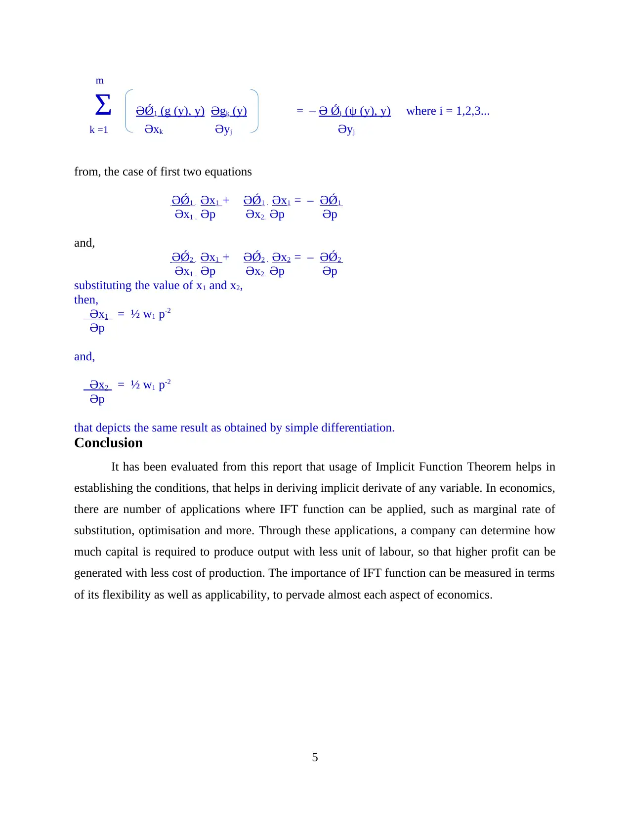
This report delves into the application of the Implicit Functional Theorem (IFT) within the field of economics. It begins by defining IFT as a tool for transforming relations into functions of multiple real variables, providing sufficient conditions for such transformations. The report then explores the use of IFT in economic contexts, specifically examining its merits. It uses two case studies to illustrate the application of IFT. The first case analyzes the relationship between labor and capital in production through isoquant functions, demonstrating how IFT can help measure the substitution rate between capital and labor. The second case examines profit maximization using production functions, showing how IFT can be used to derive implicit derivatives and optimize outputs based on input costs and prices. The report concludes by highlighting the flexibility and applicability of IFT across various economic aspects, such as marginal rates of substitution and optimization, emphasizing its importance in determining optimal production strategies and maximizing profits. The report also includes references to relevant academic sources.

ASSESSMENT

TABLE OF CONTENTS
INTRODUCTION...........................................................................................................................1
Application of IFT in economics.....................................................................................................1
A Merits of using IFT in economics............................................................................................1
Conclusion.......................................................................................................................................5
REFERENCES................................................................................................................................6

INTRODUCTION
Implicit Functional Theorem refers to a tool which allows relations to be transformed into
functions of multiple real variables (Magnus and Neudecker, 2019). This is done by representing
relations as graph of functions. It is done by representing the relations as graph of functions.
There is not single function the graph of which could be represented by the entire relations there
could be such functions on restriction of domain of relations (Agler, 2016). It gives sufficient
conditions for ensuring that there exists such functions. The present report is going to explore the
use of IFT theorem in economics, with a number of illustrations to determine major benefits of
same as well.
Application of IFT in economics
A Merits of using IFT in economics
The functional theorem allows economists in finding the relationship between the
variables of productions in a slope form (Baldi and Haus, 2017). Usage of Implicit Functional
Theorem in economics, a company can analyse conditions to maximise its profit with less capital
and labour requirements.
To examine the merits of applying IFT in economical problems, take an example of two
variables related with productions in a firm (Magnus and Neudecker, 2019). It includes labour
and capital, which are considered as main aspects for producing a commodity. Hereby, capital is
defined as cash which is used for producing goods while, labour refers to amount of work for the
same.
Case I
Problem Statement of Case I
Consider a firm uses capital K and labour L as two main functions, then relationship
between two variables that are labour and capital in production, can be defined by a function in
following way –
Q = F (L, K)
where, L represents labour and K denotes capital
the level curve of this function at equal production, can be defined as Isoquant function –
Q0 = F (L, K)
Differentiating this function partially with respect to L, result will be –
ӘQ + ӘQ . ӘK = 0
ӘL ӘK ӘL
or,
1

∆Q = ӘQ . ∆L + ӘQ . ∆K
ӘL ӘK
here, partial derivate ӘK / ӘL helps in measuring substitution rate of capital, required by labour
in order to keep the production output constant.
Now, keeping the Q (quantity) fixed and assuming K as a function of L then,
taking limits of continuity as –
Lim (∆L, ∆k) → (0,0) ∆Q = ӘQ
= ӘQ . ӘL + ӘQ . ӘK
ӘL ӘK
while, along an isoquant –
0 = ӘQ . ӘL + ӘQ . ӘK
ӘL ӘK
or,
ӘK = – ӘQ/ ӘL
ӘL ӘQ/ ӘK
It has been interpreted from this relationship that marginal rate of capital substitution in context
with labour, will be reflected as constant multiple of average capital for labour.
2

Case II
Problem Statement of Case II : Let a company produces outputs by using a single input x at
cost w with price p, using production function f, its profit can be determined by
π(x,(w, p) = pf(x) – wx.
While, maximum profit can be measured by differentiating the given function as –
π' (w,p) = pf(x'(w,p)) - w x' (w,p)
here, π denotes profit and x'(w,p) indicates optimal output at price (w,p) of input.
Example – Let production function of a firm with two variables x1 and x2, as
y = 12x1 + 10 x2 – x21 – x22 ...(1)
then, profit function of this firm can be given by –
π = py – w1 x1 – w2 x2
= p (12x1 + 10 x2 – x21 – x22) – w1 x1 – w2 x2 ...(2)
where, p is price and w1 and w2 are the costs of units,
then, first order conditions at which profit maximisation can be applied as –
π = 12px1 + 10px2 – px21 – px22 – w1 x1 – w2 x2
Differentiating with respect to x1,
Әπ = Ǿ1 = 12p – 2px1 – w1= 0 ...(3)
Әx1
Differentiating with respect to x2,
Әπ = Ǿ2 = 10p – 2px2 – w2= 0 ...(4)
Әx2
solving the (3) equation, we get
x1 = 6 – w1/2p
and,
solving the (4) equation, we get
x2 = 5 – w2/2p
the derivatives of x1 and x2,
x1 = 6 – ½ w1 p-1
x2 = 5 – ½ w2 p-1
3

again, differentiating the above equation with respect to p,
Әx1 = ½ w1 p-2
Әp
and, with respect to w1,
Әx1 = – ½ p-1
Әw1
while, with respect to w2
Әx1 = 0
Әw2
Similarly,
Әx2 = ½ w2 p-2
Әp
and, with respect to w1,
Әx2 = – ½ p-1
Әw2
while, with respect to w2
Әx2 = 0
Әw2
Similarly,
using Implicit Function theorem, two implicit equation of given function can be obtained as –
Ǿ1 (x1 , x2 , p, w1, w2) = 12p – 2px1 – w1= 0
Ǿ2 (x1 , x2 , p, w1, w2) = 10p – 2px2 – w2= 0
Using, Jacobian System,
ӘǾ1 ӘǾ1
Әx1 Әx2
J =
ӘǾ2 ӘǾ2
Әx1 Әx2
= -2p 0
0 -2p
The determinant of this function is 4p2 that gives positive result, therefore, Implicit Functional
theorem can easily be applied on given function as –
4

m
Σ ӘǾ1 (g (y), y) Әgk (y) = – Ә Ǿi (ψ (y), y) where i = 1,2,3...
k =1 Әxk Әyj Әyj
from, the case of first two equations
ӘǾ1 . Әx1 + ӘǾ1 . Әx1 = – ӘǾ1
Әx1 . Әp Әx2. Әp Әp
and,
ӘǾ2 . Әx1 + ӘǾ2 . Әx2 = – ӘǾ2
Әx1 . Әp Әx2. Әp Әp
substituting the value of x1 and x2,
then,
Әx1 = ½ w1 p-2
Әp
and,
Әx2 = ½ w1 p-2
Әp
that depicts the same result as obtained by simple differentiation.
Conclusion
It has been evaluated from this report that usage of Implicit Function Theorem helps in
establishing the conditions, that helps in deriving implicit derivate of any variable. In economics,
there are number of applications where IFT function can be applied, such as marginal rate of
substitution, optimisation and more. Through these applications, a company can determine how
much capital is required to produce output with less unit of labour, so that higher profit can be
generated with less cost of production. The importance of IFT function can be measured in terms
of its flexibility as well as applicability, to pervade almost each aspect of economics.
5

REFERENCES
Books and Journals
Agler, J., 2016. The implicit function theorem and free algebraic sets. Transactions of the
American Mathematical Society. 368(5). pp.3157-3175.
Baldi, P. and Haus, E., 2017. A Nash–Moser–Hörmander implicit function theorem with
applications to control and Cauchy problems for PDEs. Journal of Functional
Analysis. 273(12). pp.3875-3900.
Clausen, A. and Strub, C., 2020. Reverse calculus and nested optimization. Journal of Economic
Theory, p.105019.
Gama, A. and Rietzke, D., 2019. Monotone comparative statics in games with non-monotonic
best-replies: Contests and Cournot oligopoly. Journal of Economic Theory, 183, pp.823-
841.
Lott, S., 2019. Perturbations in DSGE models: An odd derivatives theorem. Journal of
Economic Dynamics and Control, 106, p.103722.
Magnus, J. R. and Neudecker, H., 2019. Matrix differential calculus with applications in
statistics and econometrics. John Wiley & Sons.
Rothe, C. and Wied, D., 2019. Estimating derivatives of function-valued parameters in a class of
moment condition models. Journal of Econometrics.
6