Data Analytics: Income, Age, and Social Participation Analysis Essay

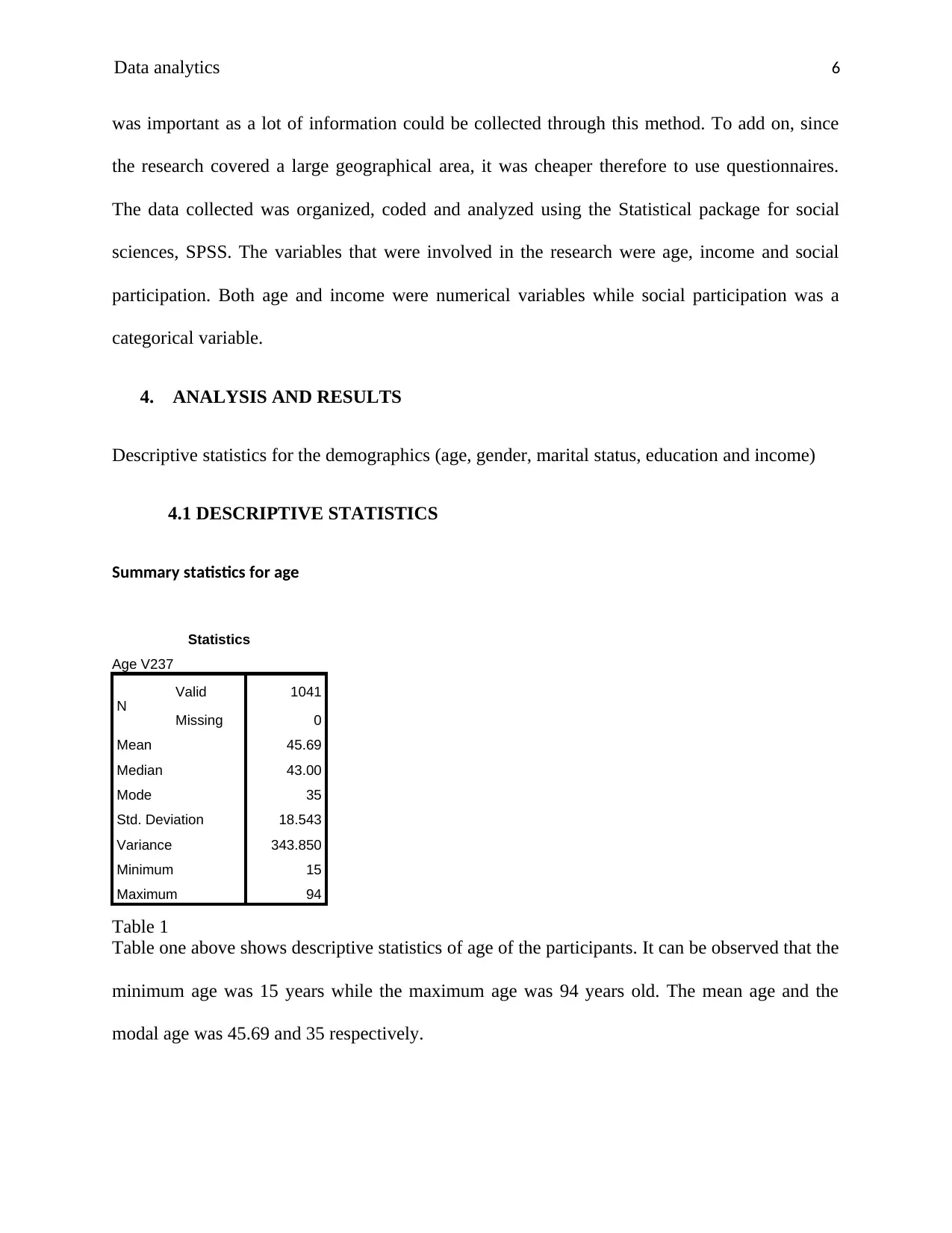
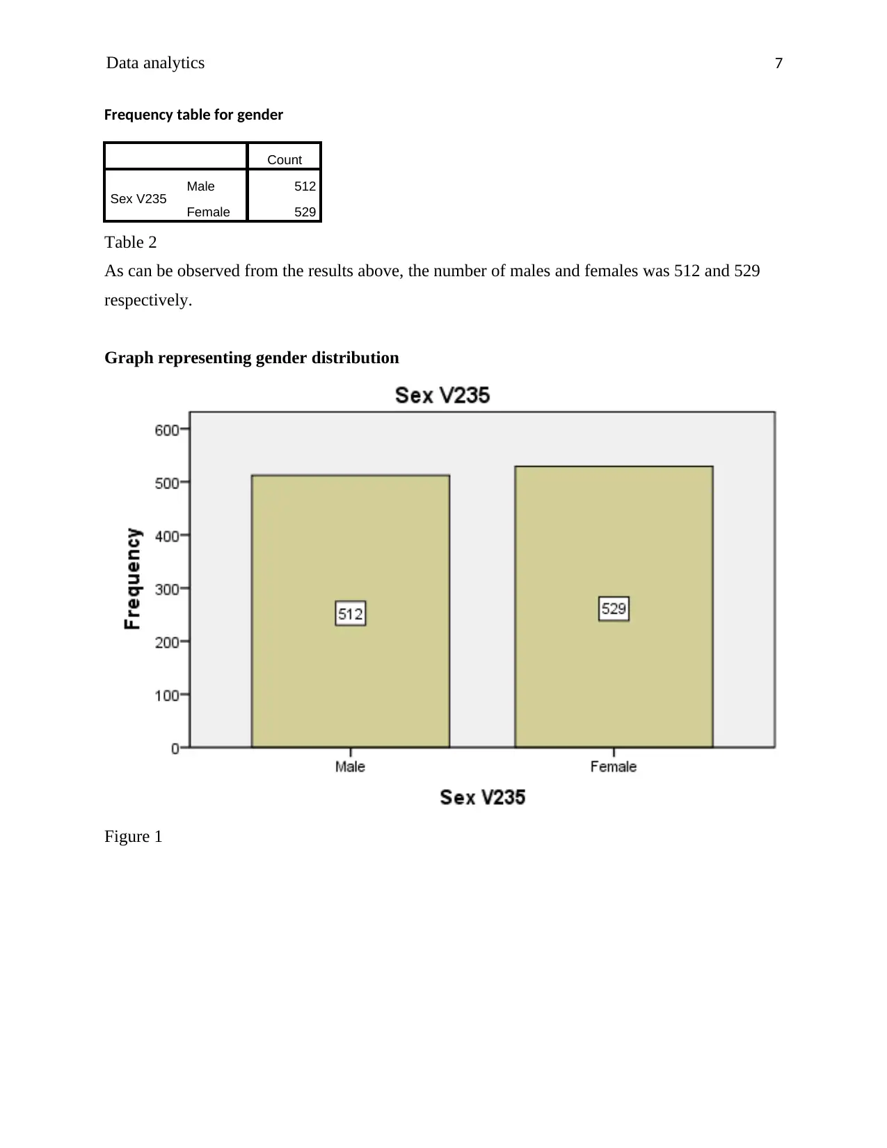
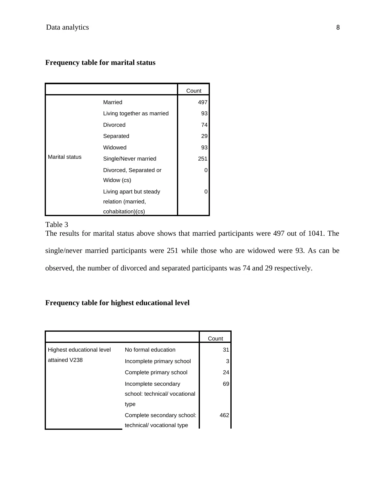
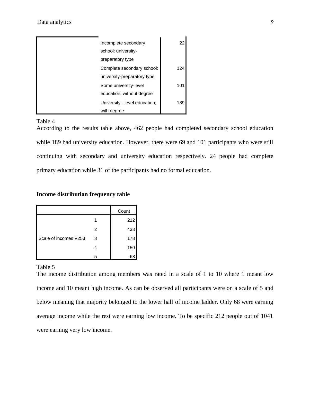
This essay investigates the relationship between income, age, and social participation using data analytics techniques. It begins with an introduction to the influence of demographic characteristics on social participation, highlighting the disparities in income across different age groups and its impact on social classes. The conceptual framework establishes a link between income inequality and social participation, drawing on existing literature and survey data to formulate hypotheses about the positive relationship between income and social participation, and age and income. The research methodology outlines the descriptive research design, population sampling, and data collection methods using questionnaires from the World Values Survey. The analysis and results section presents descriptive statistics for demographics such as age, gender, marital status, education, and income, followed by correlation and regression analyses to test the hypotheses. The essay concludes by discussing the findings and their implications for understanding the complex interplay between income, age, and social engagement. Desklib provides access to this essay and a wealth of study resources for students.

Data analytics 1
Student Name:
Student number:
Lecturer

Data analytics 2
1. INTRODUCTION
Demographic characteristic such as the level of income and age play a vital role in influencing
human beings social participation in the society. It is hypothesized that age sometimes have an
impact on an individual income. This perception is held true partially since old age is associated
with more years of working hence more accumulation of income. On the other hand, tender age
is associated with aggressiveness and energy thus being able to earn more income at one
particular time. This case can also be argued from the spending perspective. Research has shown
it that elderly people since to scale down their spending on various bills. This has been attributed
to the fact that the elderly has less years or energy to make more income. However, the same
research found that young people tend to have higher spending on their bills since they feel they
have the luxury of time to make more money. A totally different scenario plays out in some
economies. For example, in the United States, it was found that the distribution of income over
age is normal. The age group below 25 years was found to earn less. The income rose up to the
ages of between 45 and 54 after which the income seemed to fall gradually as the age decreased.
As a result of disparity in income across the ages, social classes have been created. The social
classes have in turn influenced how people participate socially in the society. In summary, it is
tempting to conclude that income influence social participation in a community. The effect of the
disparity in income in some economies has been so much so that it has been a center of political
discussions in most nations of the world just to mention the worst case scenario. High income
level has been associated with high self-esteem and the converse is also true. Due to this
participation in social forums in the community such as politics, welfare groups, religious groups
and social trust funds have been affected. There has been a skewed participation in terms of
social cadre. Low income earners due their low self-esteem think that they are inferior and so is

Data analytics 3
their opinion. They believe that only the high income earners can be heard in these forums and
their ideas implemented. It is against this background that this research study sought to establish
whether there is a relationship between income, age and social participation. The following
sections of this research will include conceptual framework, methodology, data analysis,
discussions and conclusions.
2. CONCEPTUAL FRAMEWORK
An association has been found to exist between income inequality and social participation. This
has been proven through its manifestation in various social forums. For example this has been
attributed to upsurge in the number of people who participate in politics (Solt, 2008). A political
research by (Verba et al. 1995; Scholzman, 2012) found that people who were high in terms of
socio-economic status participated more and consistently in issues that shape the country like
politics than their counterparts who are at the lowest in the socio-economic ladder. To add on,
societies which are diverse in terms of their economies participate more in civic processes
(Oliver, 1999). Income in society has also affected the level of trust or mistrust in societies.
Scholar (Hetherington, 2005) found that there was a strong correlation between decreased trust
and decreased social participation. Low social trust was also evident at the government level
where there was income inequality (Ulsaner & Brown, 2005). According to (Omoto & Synder,
2002), there is a psychological idea in the society that fulfillment, membership and integration
are paramount. This however normally affected due to inequality due to income. This further
causes a decrease in social participation since some of the members of the community always
feel that they do not fully belong due to their low income earning status. This discussion brings
the research survey to the following hypothesis;

Data analytics 4
1. There is a positive relationship between income and social participation
2. There is a positive relationship between age and income.
Conceptual framework
The research survey in the development of conceptual framework considered factors from the
literature review and the questionnaire which were used by the research study. The factor
variables will be educational factor, age factor, marital status factor, gender and satisfaction. The
main dependent variable will be organizational commitment.
Conceptual framework
{Independent variable} {Dependent variable}
3.
4.
{Independent variable} {Dependent variable}
Figure 1 Conceptual framework for the study (Source: Researcher, 2018)
3. RESEARCH METHODOLOGY
This section covers in general the methods that have been used in the research. It provides
detailed information of how the data was collected, the data collection tool, sampling techniques,
the target population, research design and sample size. To add on it highlights how the data
analysis and various reliability and validity tests were done.
AGE INCOME
SOCIAL
PARTICIPATIONINCOME

Data analytics 5
3.1 RESEARCH DESIGN
Choosing a suitable design in this research was considered a very key step in the study. This is
because an appropriate research design presents an exhaustive description of relevant
components of the research study. Since this research study was based on data collected rather
than either assumptions or predictions, it majorly used descriptive research design. It was a
single cross-sectional descriptive approach that covered members of the public. This approach
was appropriate because the study participants were studied at one particular time rather than for
a length of time. In addition, according to (Mannion, 1994), this research design allows the
researcher to collect data from large number of respondents. On the other hand, (Coopers &
Emory, 1995) applaud this method for its suitability to get first-hand information from the
respondents. This approach also allowed the research to be able to compare the effect of a single
variable on various dependent variables of the study; for example in this study, the extent of
effect of age on income and the effect of income on social participation.
3.2 POPULATION AND SAMPLING.
The target population was members of the public who were above 18 years old and above.
Simple random sampling or equal probability sampling was employed to recruit participants. The
research found this method appropriate as it gave each member of the public an equal chance of
being selected in the sample.
3.3 DATA COLLECTION
This research used questionnaires to collect data through world value survey wave. Primary data
was important to this survey as it provided the study with first-hand information about
interaction of variables such as age, income and social participation. The use of questionnaire

Data analytics 6
was important as a lot of information could be collected through this method. To add on, since
the research covered a large geographical area, it was cheaper therefore to use questionnaires.
The data collected was organized, coded and analyzed using the Statistical package for social
sciences, SPSS. The variables that were involved in the research were age, income and social
participation. Both age and income were numerical variables while social participation was a
categorical variable.
4. ANALYSIS AND RESULTS
Descriptive statistics for the demographics (age, gender, marital status, education and income)
4.1 DESCRIPTIVE STATISTICS
Summary statistics for age
Statistics
Age V237
N Valid 1041
Missing 0
Mean 45.69
Median 43.00
Mode 35
Std. Deviation 18.543
Variance 343.850
Minimum 15
Maximum 94
Table 1
Table one above shows descriptive statistics of age of the participants. It can be observed that the
minimum age was 15 years while the maximum age was 94 years old. The mean age and the
modal age was 45.69 and 35 respectively.

Data analytics 7
Frequency table for gender
Count
Sex V235 Male 512
Female 529
Table 2
As can be observed from the results above, the number of males and females was 512 and 529
respectively.
Graph representing gender distribution
Figure 1

Data analytics 8
Frequency table for marital status
Count
Marital status
Married 497
Living together as married 93
Divorced 74
Separated 29
Widowed 93
Single/Never married 251
Divorced, Separated or
Widow (cs)
0
Living apart but steady
relation (married,
cohabitation)(cs)
0
Table 3
The results for marital status above shows that married participants were 497 out of 1041. The
single/never married participants were 251 while those who are widowed were 93. As can be
observed, the number of divorced and separated participants was 74 and 29 respectively.
Frequency table for highest educational level
Count
Highest educational level
attained V238
No formal education 31
Incomplete primary school 3
Complete primary school 24
Incomplete secondary
school: technical/ vocational
type
69
Complete secondary school:
technical/ vocational type
462

Data analytics 9
Incomplete secondary
school: university-
preparatory type
22
Complete secondary school:
university-preparatory type
124
Some university-level
education, without degree
101
University - level education,
with degree
189
Table 4
According to the results table above, 462 people had completed secondary school education
while 189 had university education. However, there were 69 and 101 participants who were still
continuing with secondary and university education respectively. 24 people had complete
primary education while 31 of the participants had no formal education.
Income distribution frequency table
Count
Scale of incomes V253
1 212
2 433
3 178
4 150
5 68
Table 5
The income distribution among members was rated in a scale of 1 to 10 where 1 meant low
income and 10 meant high income. As can be observed all participants were on a scale of 5 and
below meaning that majority belonged to the lower half of income ladder. Only 68 were earning
average income while the rest were earning low income. To be specific 212 people out of 1041
were earning very low income.

Data analytics
10
Figure 2
4.2 CORRELATION ANALYSIS
a. Correlation between income and age
Correlations
Age V237 Scale of
incomes V253
Age V237
Pearson Correlation 1 .131**
Sig. (2-tailed) .000
N 1041 1041
Scale of incomes V253
Pearson Correlation .131** 1
Sig. (2-tailed) .000
N 1041 1041

Data analytics
11
**. Correlation is significant at the 0.01 level (2-tailed).
Table 6
The table above shows the correlation results between age and income. It can be observed that
the Pearson correlation coefficient is 0.131. This shows a weak but positive correlation between
the two variables.
b. Correlation between income and social participation
Correlations
Scale of
incomes V253
Membership in
voluntary
organizations.
Added V23 to
V33
Scale of incomes V253
Pearson Correlation 1 -.190**
Sig. (2-tailed) .000
N 1041 981
Membership in voluntary
organizations. Added V23 to
V33
Pearson Correlation -.190** 1
Sig. (2-tailed) .000
N 981 981
**. Correlation is significant at the 0.01 level (2-tailed).
Table 7
The table above shows the correlation results between social participation and income. It can be
observed that the Pearson correlation coefficient is -0.19. This shows a weak and negative
correlation between the two variables.

Data analytics
12
4.3 REGRESSION ANALYSIS
a. Age and income
Independent variable: Age
Dependent variable: Income
Results tables
Model Summary
Model R R Square Adjusted R
Square
Std. Error of the
Estimate
1 .131a .017 .016 1.147
a. Predictors: (Constant), Age V237
Table 8
ANOVAa
Model Sum of Squares df Mean Square F Sig.
1
Regression 23.944 1 23.944 18.214 .000b
Residual 1365.856 1039 1.315
Total 1389.800 1040
a. Dependent Variable: Scale of incomes V253
b. Predictors: (Constant), Age V237
Table 9
Coefficientsa
Model Unstandardized Coefficients Standardized
Coefficients
t Sig.
B Std. Error Beta
1 (Constant) 2.078 .095 21.979 .000
Age V237 .008 .002 .131 4.268 .000
a. Dependent Variable: Scale of incomes V253
Table 10
Table 8, 9 and 10 are results are regression results for age and income. From table 8, it can be
observed that the value of R-square is 0.017. This indicates that only 1.7% of the variation in the