Income Distribution Analysis: Kaggle Dataset and Statistical Analysis
VerifiedAdded on 2022/09/14
|16
|2079
|9
Report
AI Summary
This report presents an analysis of income distribution in Australia, using a dataset collected from Kaggle and analyzed in Excel. The study explores the relationships between income levels and customer spending and purchasing behaviors. The report includes descriptive statistics, regression analysis, and graphical representations such as scatter plots and box plots to visualize the data and draw conclusions. The analysis examines the impact of income on various factors, including clicks, last spend, and purchases, considering both numeric and categorical variables. The findings reveal insights into spending patterns and highlight the influence of education and experience on income levels. The report concludes by summarizing key observations and emphasizing the importance of considering multiple factors beyond age and experience when assessing income distribution.

INCOME 1
TOPIC
NAME OF AUTHOR
NAME OF PROFESSOR
NAME OF CLASS
NAME OF SCHOOL
STATE AND CITY OF SCHOOL
TOPIC
NAME OF AUTHOR
NAME OF PROFESSOR
NAME OF CLASS
NAME OF SCHOOL
STATE AND CITY OF SCHOOL
Paraphrase This Document
Need a fresh take? Get an instant paraphrase of this document with our AI Paraphraser
INCOME 2
Executive Summary
This will be written literature on income distribution. Data was to be collected and with at least
50 cases or observations, at least two numeric variables and at least two categorical variables.
Every other student that was to participate in this exercise, had full liberty of choosing the actual
topic to write on from this list; Recycling, Tourism, Distribution of income, Food and Beveridge
industries, Volunteering, Humanitarian Agencies and NGOs, Indigenous perspectives (other than
health) and Indigenous perspectives (other than crime-related). As for this literature, as indicated,
the topic that was chosen was income distribution. An Australian dataset was collected on
income distribution and this dataset was to be used for analysis. The analysis was to be done in
excel, the actual software where the dataset was to be collected and stored for analysis. The
collected dataset had variables; CustNum (customer number), Sex, State, Age, Income, Clicks,
LastSpend, Purchases, Spend. In this case, there are more numeric variables than was required.
The entirety of the dataset will be spoken about in the subsequent sections. The next section will
be the introduction section, which will tend to explain matters related to the dataset in more
details. After that, there will be a direct dive into actual analysis and the interpretation of the
results that have been derived from the whole analysis of the dataset that was collected.
Alongside analysis interpretation, there will be graphical displays both in the body of the
literature as well as, the appendix section.
A summary and conclusion will wrap up the literature content after which, the appendix section,
will contain all the graphs and analysis results that could not be included in the main body of
literature.
INCOME 3
Introduction (Methods used to collect and Collate External Data)
Of the topics that were mentioned in the executive summary area, one of them was to be chosen.
For our analysis and literature, we chose the income distribution topic. A dataset was also
collected for the same and what needed to be looked into was the effects of the distribution of
income on different customers from Australia and how their purchasing and spending habits
were when it came to income levels.
The actual source of the dataset was the Kaggle website. The dataset had up to 1000 cases but for
simplicity of analysis and better understanding, cleaning was done on the very same dataset and
therefore only three hundred cases were left. This is what later was run in for analysis.
The actual purpose of this exercise is to be able to tell a story using an actual sample dataset.
Like a story, we are supposed to use our dataset to create an account of events that is a true
representation of the whole society.
As it is known, most people earn, in most societies, earnings, is directly proportional to age in
that as age increases, the amounts that other ear also increases as it is believed that, if an
individual has been serving at a role, then over time, their experiences, are only bound to grow
warranting them an increase in salary. But in others what would largely propel your earning
increment are two factors combined, your level of education as well as your experience level in a
field. Just as the saying goes, money changes people, so is the level of income bound to change
the way an individual spends his or her money altogether, purchasing habits, amounts spent and
all. In our dataset, there are different characters and different spending habits with different
incomes. Different things are resulted by the amounts earned and in this case, the main
⊘ This is a preview!⊘
Do you want full access?
Subscribe today to unlock all pages.
Trusted by 1+ million students worldwide
INCOME 4
independent variable, meaning it determines the number of clicks an individual will have to
make while searching for a good online. The level of income again determines the number of
purchase. In an area where there is a high amount of income and yet, purchases are low, then the
only resolution that can be made is that, the individual might be having other uses with funds, ad
these might be related to paying school fees for kids, paying for own school fees among other
responsibilities, which little room for more cash in hand hence less spending and fewer
purchases. Others are younger and yet earn the same as their older fellows or even more. This is
where we get to include both experience and academic advancement in determining the amount
and individual earns and not only focus on years of experience alone.
Analysis and Interpretation (Key Concepts in Statistics and Probability in Drawing
Conclusions from Analysis.
i. Descriptive Analysis
The very first analysis that we will be focusing on, will be the descriptive analysis. Descriptive
analysis is highly elaborative on numeric variables as opposed to categorical variables. The
actual descriptive on six numeric variables will be;
Paraphrase This Document
Need a fresh take? Get an instant paraphrase of this document with our AI Paraphraser
INCOME 5
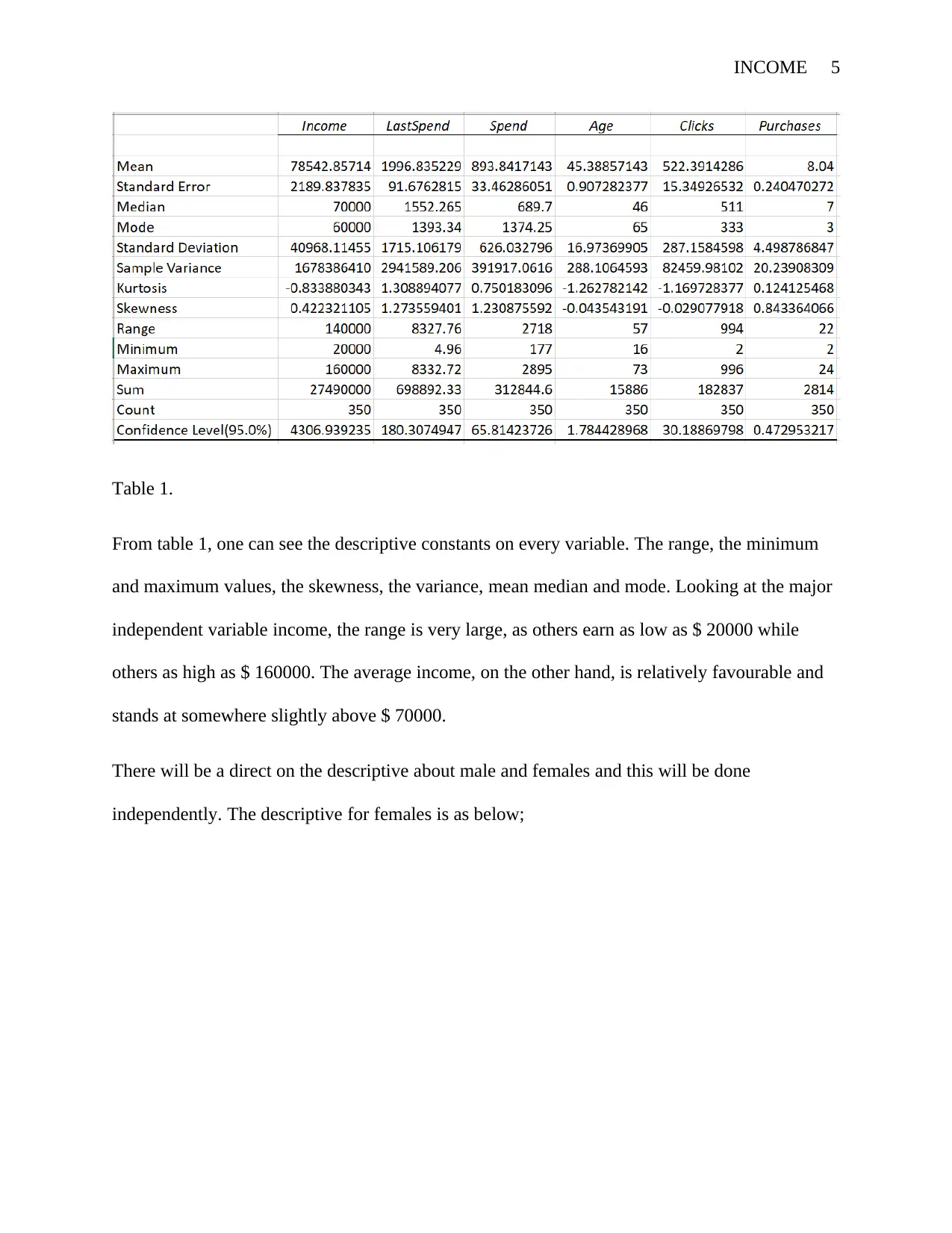
Table 1.
From table 1, one can see the descriptive constants on every variable. The range, the minimum
and maximum values, the skewness, the variance, mean median and mode. Looking at the major
independent variable income, the range is very large, as others earn as low as $ 20000 while
others as high as $ 160000. The average income, on the other hand, is relatively favourable and
stands at somewhere slightly above $ 70000.
There will be a direct on the descriptive about male and females and this will be done
independently. The descriptive for females is as below;
INCOME 6
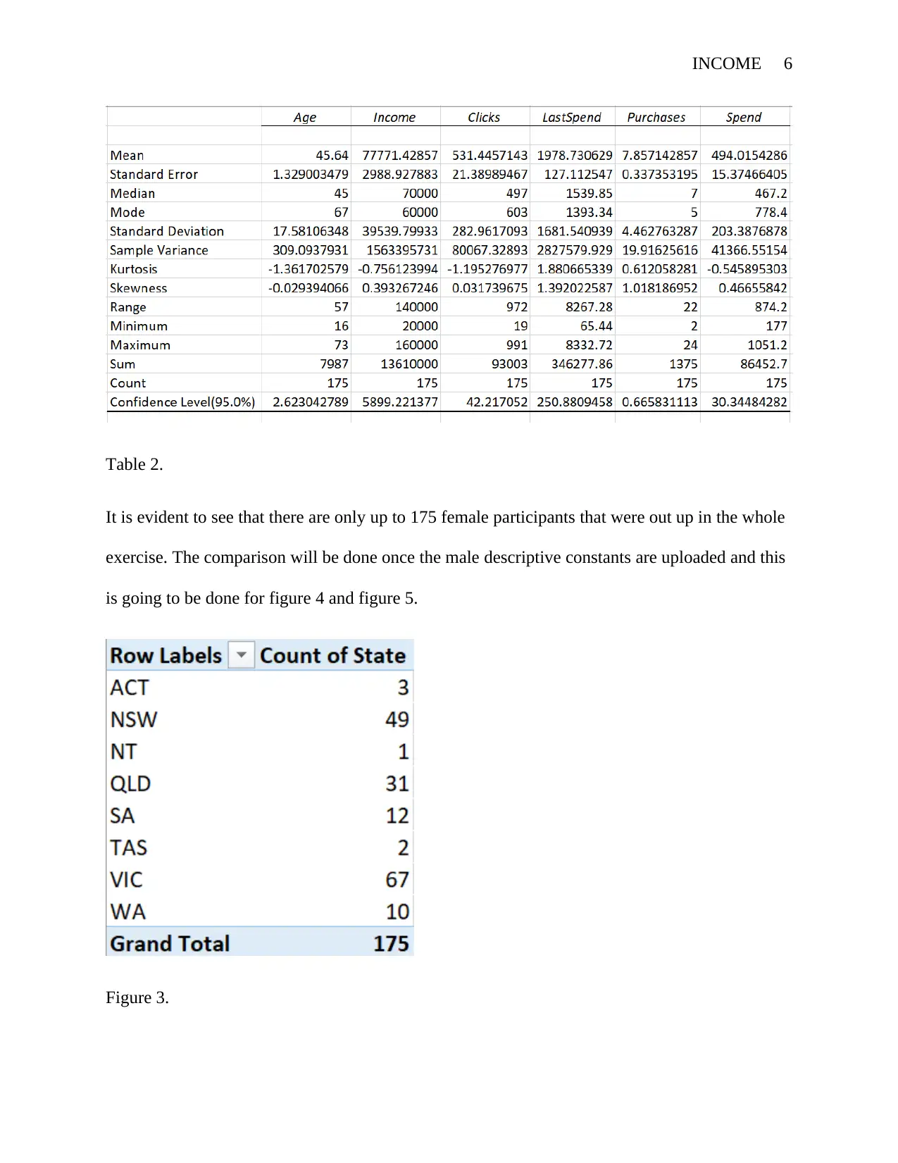
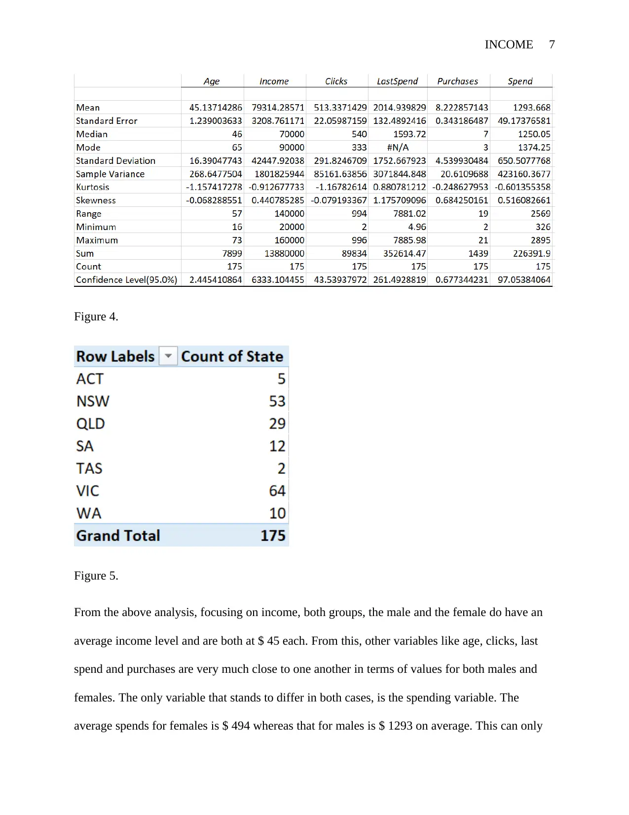
Table 2.
It is evident to see that there are only up to 175 female participants that were out up in the whole
exercise. The comparison will be done once the male descriptive constants are uploaded and this
is going to be done for figure 4 and figure 5.
Figure 3.
Table 2.
It is evident to see that there are only up to 175 female participants that were out up in the whole
exercise. The comparison will be done once the male descriptive constants are uploaded and this
is going to be done for figure 4 and figure 5.
Figure 3.
⊘ This is a preview!⊘
Do you want full access?
Subscribe today to unlock all pages.
Trusted by 1+ million students worldwide
INCOME 7
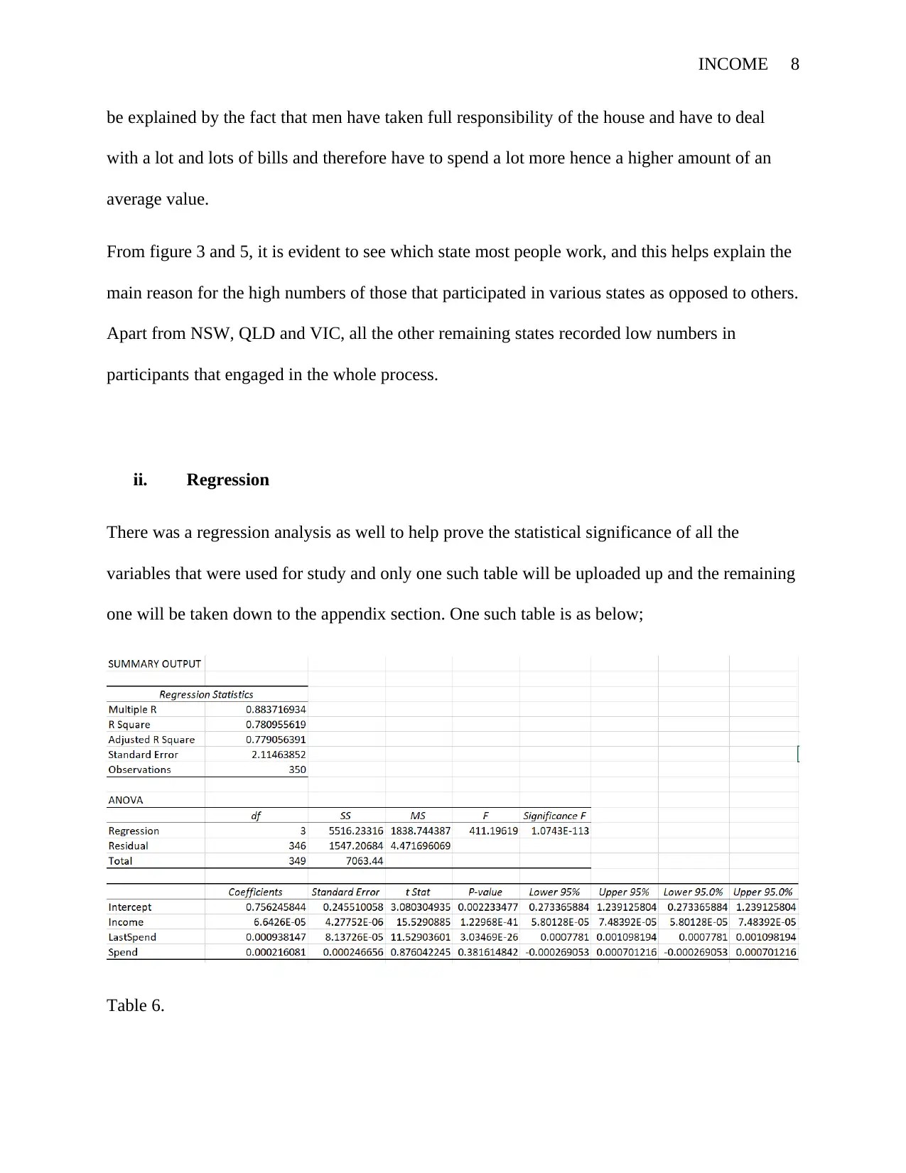
Figure 4.
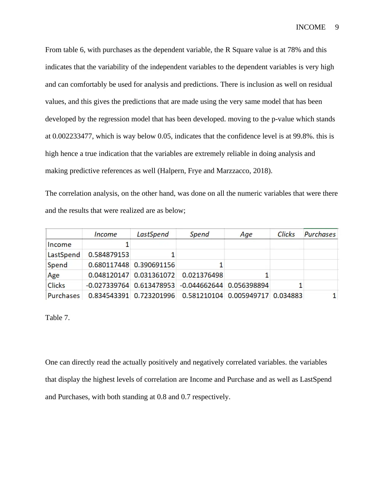
Figure 5.
From the above analysis, focusing on income, both groups, the male and the female do have an
average income level and are both at $ 45 each. From this, other variables like age, clicks, last
spend and purchases are very much close to one another in terms of values for both males and
females. The only variable that stands to differ in both cases, is the spending variable. The
average spends for females is $ 494 whereas that for males is $ 1293 on average. This can only
Figure 4.
Figure 5.
From the above analysis, focusing on income, both groups, the male and the female do have an
average income level and are both at $ 45 each. From this, other variables like age, clicks, last
spend and purchases are very much close to one another in terms of values for both males and
females. The only variable that stands to differ in both cases, is the spending variable. The
average spends for females is $ 494 whereas that for males is $ 1293 on average. This can only
Paraphrase This Document
Need a fresh take? Get an instant paraphrase of this document with our AI Paraphraser
INCOME 8
be explained by the fact that men have taken full responsibility of the house and have to deal
with a lot and lots of bills and therefore have to spend a lot more hence a higher amount of an
average value.
From figure 3 and 5, it is evident to see which state most people work, and this helps explain the
main reason for the high numbers of those that participated in various states as opposed to others.
Apart from NSW, QLD and VIC, all the other remaining states recorded low numbers in
participants that engaged in the whole process.
ii. Regression
There was a regression analysis as well to help prove the statistical significance of all the
variables that were used for study and only one such table will be uploaded up and the remaining
one will be taken down to the appendix section. One such table is as below;
Table 6.
INCOME 9
From table 6, with purchases as the dependent variable, the R Square value is at 78% and this
indicates that the variability of the independent variables to the dependent variables is very high
and can comfortably be used for analysis and predictions. There is inclusion as well on residual
values, and this gives the predictions that are made using the very same model that has been
developed by the regression model that has been developed. moving to the p-value which stands
at 0.002233477, which is way below 0.05, indicates that the confidence level is at 99.8%. this is
high hence a true indication that the variables are extremely reliable in doing analysis and
making predictive references as well (Halpern, Frye and Marzzacco, 2018).
The correlation analysis, on the other hand, was done on all the numeric variables that were there
and the results that were realized are as below;
Table 7.
One can directly read the actually positively and negatively correlated variables. the variables
that display the highest levels of correlation are Income and Purchase and as well as LastSpend
and Purchases, with both standing at 0.8 and 0.7 respectively.
⊘ This is a preview!⊘
Do you want full access?
Subscribe today to unlock all pages.
Trusted by 1+ million students worldwide
INCOME 10
Graphical and Visual representation of data.
i. Scatter plot
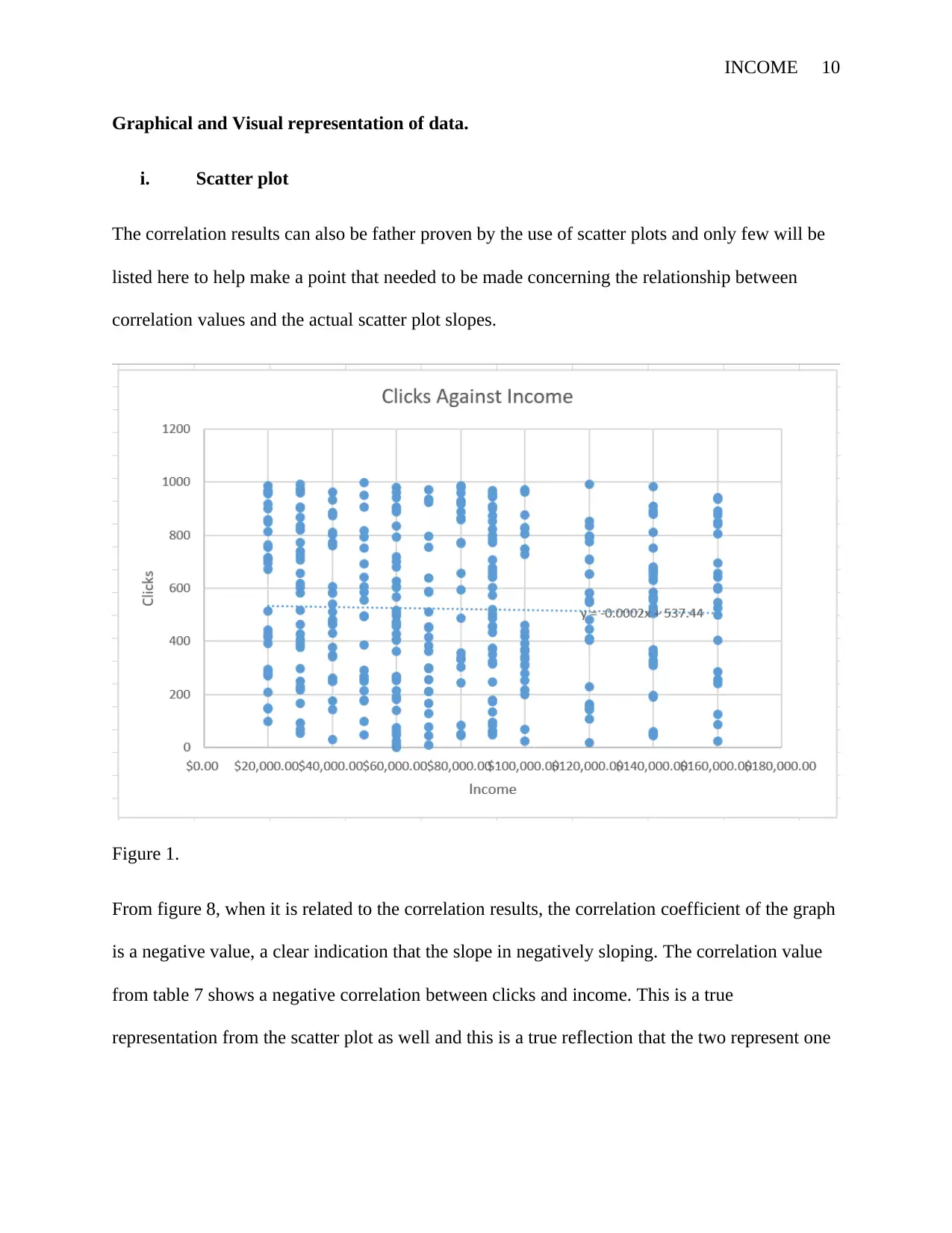
The correlation results can also be father proven by the use of scatter plots and only few will be
listed here to help make a point that needed to be made concerning the relationship between
correlation values and the actual scatter plot slopes.
Figure 1.
From figure 8, when it is related to the correlation results, the correlation coefficient of the graph
is a negative value, a clear indication that the slope in negatively sloping. The correlation value
from table 7 shows a negative correlation between clicks and income. This is a true
representation from the scatter plot as well and this is a true reflection that the two represent one
Graphical and Visual representation of data.
i. Scatter plot
The correlation results can also be father proven by the use of scatter plots and only few will be
listed here to help make a point that needed to be made concerning the relationship between
correlation values and the actual scatter plot slopes.
Figure 1.
From figure 8, when it is related to the correlation results, the correlation coefficient of the graph
is a negative value, a clear indication that the slope in negatively sloping. The correlation value
from table 7 shows a negative correlation between clicks and income. This is a true
representation from the scatter plot as well and this is a true reflection that the two represent one
Paraphrase This Document
Need a fresh take? Get an instant paraphrase of this document with our AI Paraphraser
INCOME 11
another. In summary, a negative correlation value shows that the gradient of the graph is
negative and vice versa. The remaining scatter plots will be shown in the appendix section.
ii. Box plot
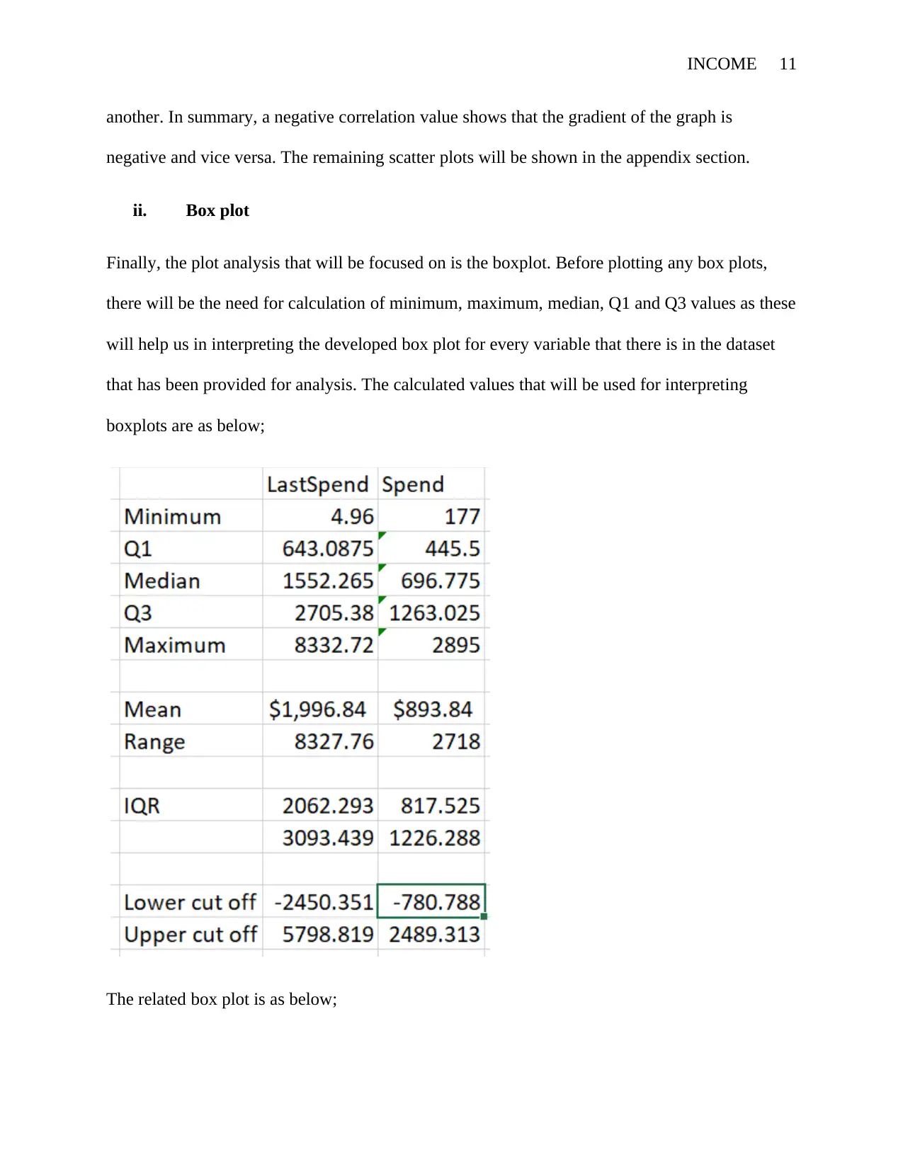
Finally, the plot analysis that will be focused on is the boxplot. Before plotting any box plots,
there will be the need for calculation of minimum, maximum, median, Q1 and Q3 values as these
will help us in interpreting the developed box plot for every variable that there is in the dataset
that has been provided for analysis. The calculated values that will be used for interpreting
boxplots are as below;
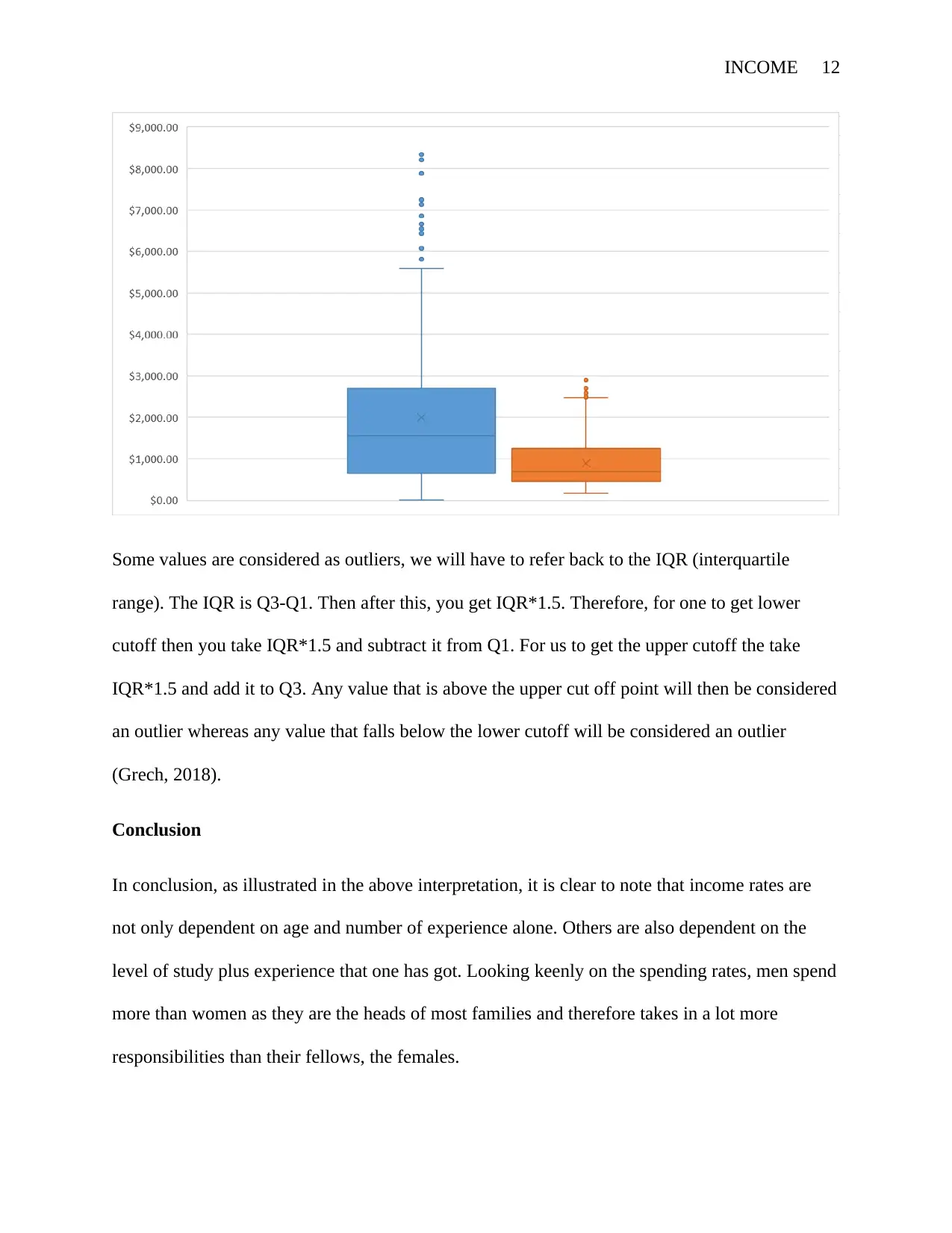
The related box plot is as below;
another. In summary, a negative correlation value shows that the gradient of the graph is
negative and vice versa. The remaining scatter plots will be shown in the appendix section.
ii. Box plot
Finally, the plot analysis that will be focused on is the boxplot. Before plotting any box plots,
there will be the need for calculation of minimum, maximum, median, Q1 and Q3 values as these
will help us in interpreting the developed box plot for every variable that there is in the dataset
that has been provided for analysis. The calculated values that will be used for interpreting
boxplots are as below;
The related box plot is as below;
INCOME 12
Some values are considered as outliers, we will have to refer back to the IQR (interquartile
range). The IQR is Q3-Q1. Then after this, you get IQR*1.5. Therefore, for one to get lower
cutoff then you take IQR*1.5 and subtract it from Q1. For us to get the upper cutoff the take
IQR*1.5 and add it to Q3. Any value that is above the upper cut off point will then be considered
an outlier whereas any value that falls below the lower cutoff will be considered an outlier
(Grech, 2018).
Conclusion
In conclusion, as illustrated in the above interpretation, it is clear to note that income rates are
not only dependent on age and number of experience alone. Others are also dependent on the
level of study plus experience that one has got. Looking keenly on the spending rates, men spend
more than women as they are the heads of most families and therefore takes in a lot more
responsibilities than their fellows, the females.
⊘ This is a preview!⊘
Do you want full access?
Subscribe today to unlock all pages.
Trusted by 1+ million students worldwide
1 out of 16


Your All-in-One AI-Powered Toolkit for Academic Success.
+13062052269
info@desklib.com
Available 24*7 on WhatsApp / Email
![[object Object]](/_next/static/media/star-bottom.7253800d.svg)
Unlock your academic potential
Copyright © 2020–2026 A2Z Services. All Rights Reserved. Developed and managed by ZUCOL.