Financial Distress Prediction in Indonesian Manufacturing Industry
VerifiedAdded on 2023/04/21
|22
|8279
|487
Report
AI Summary
This discussion paper, "Predicting Financial Distress in Indonesian Manufacturing Industry," by Muhammad Rifqi and Yoshio Kanazaki, explores the development and evaluation of financial distress prediction models using financial ratios from Indonesian manufacturing companies listed on the Indonesian Stock Exchange between 2003 and 2011. The study employs both traditional statistical methods (Logistic Regression and Discriminant Analysis) and a modern tool (Neural Network) to analyze 23 financial ratios related to liquidity, profitability, leverage, and cash position. The research identifies key ratios contributing to financial distress and constructs prediction models. The results indicate that the ratios identified by logistic regression and the model built on that basis is more appropriate than those derived from discriminant analysis. The paper also highlights the performance of a neural network model, while acknowledging the lack of definitive proof of its absolute superiority over traditional methods. The study uses the book value of total debt exceeding the book value of total assets as a definition of financial distress and discusses the challenges of using bankruptcy data in developing countries, which led to the focus on financial distress prediction. The paper also includes a review of existing literature, including models by Altman, Ohlson, Fulmer, and Shirata, and concludes by outlining potential areas for future research.
Data Science and Service Research
Discussion Paper
Discussion Paper No. 62
Predicting Financial Distress in Indonesian
Manufacturing Industry
MUHAMMAD RIFQI and YOSHIO KANAZAKI
June, 2016
May 2016
Center for Data Science and Service Research
Graduate School of Economic and Management
Tohoku University
27-1 Kawauchi, Aobaku
Sendai 980-8576, JAPAN
Paraphrase This Document
Need a fresh take? Get an instant paraphrase of this document with our AI Paraphraser
1
Predicting Financial Distress in Indonesian Manufacturing
Industry
MUHAMMAD RIFQI and YOSHIO KANAZAKI *
ABSTRACT
We attempt to develop and evaluate financial distress prediction models using
financial ratios derived from financial statements of companies in Indonesian
manufacturing industry. The samples are manufacturing companies listed in
Indonesian Stock Exchange during 2003-2011. The models employ two kinds of
methods: traditional statistical modeling (Logistic Regression and Discriminant
Analysis) and modern modeling tool (Neural Network). We evaluate 23 financial
ratios (that measure a company’s liquidity, profitability, leverage, and cash
position) and are able to identify a set of ratios that significantly contribute to
financial distress condition of the companies in sample group. By utilizing those
ratios, prediction models are developed and evaluated based on accuracy and
error rates to determine the best model. The result shows that the ratios
identified by logistic regression and the model built on that basis is more
appropriate than those derived from discriminant analysis. The research also
shows that although the best performing prediction model is a neural network
model, but we have no solid proof of neural network’s absolute superiority over
traditional modeling methods.
Keywords: financial distress, prediction model, discriminant analysis, logistic
regression, neural network.
1. INTRODUCTION
The topic of financial distress prediction has been attracting many researchers’ attention,
especially those in accounting field. Financial distress prediction models have been created
to cope with financial difficulties condition faced by companies, especially in post-crisis
period (Shirata, 1998). The development of prediction models started when Beaver
introduced a simple univariate analysis of financial ratios to predict future bankruptcy
(Beaver, 1966). Since then, many researchers have been struggling to develop financial
distress prediction techniques using statistical models. The most popular example was
* Graduate School of Economics and Management, Tohoku University, Sendai, Japan
This work was supported by JSPS KAKENHI Grant Number JP25380385.
2
Altman Z-Score model which utilizes 5 different financial ratios in his prediction model
(Altman, 1968). Other notable models include Ohlson model in 1980 (Ohlson, 1980), Fulmer
model in 1984 (Fulmer, 1984), and Springate model in 1978 (Springate, 1978). Besides
western researchers, accounting researchers from Asia also present their models, such as
Shirata who presented her first model in 1998 and then updating it in 2003 (the updated
version, being known as SAF2002 model, is widely used in Japan). Sung, Chang, and Lee
(1999) analyzes financial pattern and significant financial ratios to discriminate future
bankrupt companies under different macroeconomic circumstances. Bae (2012) develops a
distress prediction model based on radial basis support vector machine (RSVM) for
companies in South Korean manufacturing industry. In the case of Indonesia, there have
been several but still limited models developed by researchers to predict financial distress.
Indonesian researchers focused mainly on Indonesian manufacturing Industry, such as
Luciana (2003) and Brahmana (2005).
It is important to note that “financial distress” and “bankruptcy” is not the same thing.
Financial distress typically takes place before bankruptcy; therefore it can be considered as
an indicator of bankruptcy (Luciana, 2003). Due to the convenience in obtaining the legal
data and the relatively efficient process of bankruptcy filing, most researchers that use US
companies in their study use the legal definition of bankruptcy in their prediction models. In
other words, they classify the firms which filed for bankruptcy in legal court as the
“bankrupt” group, thus they are developing bankruptcy prediction models, not financial
distress prediction models. Same thing also applies in relatively developed countries where
the bankruptcy filing process can be conducted efficiently, such as Canada (Springate, 1978)
and Japan (Shirata, 1998). Meanwhile, some other researchers use delisting status from the
exchange as their bankruptcy proxy, for example Shumway (2001).
However, for researchers who take the companies in developing economies as their
sample, using legal definition of bankruptcy might pose a grave problem. This is due to the
fact that bankruptcy filing process in a developing country typically takes years to complete,
so it will be a long process until a company can be declared bankrupt. For example, in the
case of Indonesia, a bankruptcy filing process in court usually takes a considerably long time
to undergo, and the data of bankruptcy filing is very hard to obtain from Indonesian
Corporate Court (Zu’amah, 2005). If they decided to use the bankruptcy data for their
prediction models, there will be a significant amount of time lag between the date of
bankruptcy declaration and the financial numbers they use to predict the bankruptcy event,
thus greatly reducing the relevance of their model to predicting the bankruptcy event. Due
to this problem, the researchers in developing countries resort to an alternative strategy:
they use “financial distress” status instead of “bankruptcy” status, thus making their
⊘ This is a preview!⊘
Do you want full access?
Subscribe today to unlock all pages.
Trusted by 1+ million students worldwide
3
prediction models a little different in nature to those of developed countries. However, in
this study we will use the term “financial distress” and “bankruptcy” interchangeably.
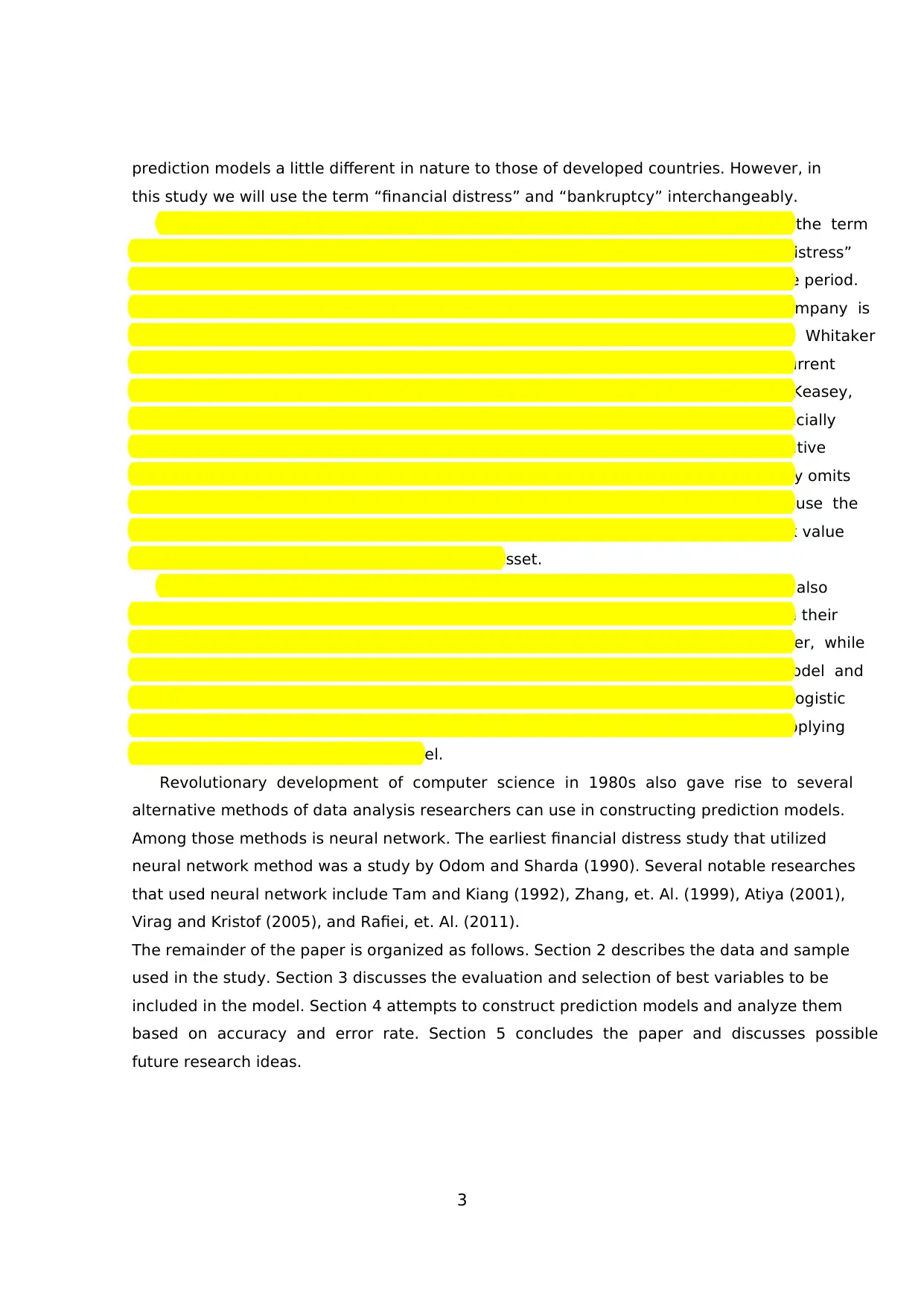
It is necessary to understand that there is no single accurate definition of the term
“financial distress” itself. Hofer (1980) as noted in Luciana (2006) defines “financial distress”
as a condition in which a company suffers from negative net income for a consecutive period.
Luciana (2006) herself defines “financial distress” as a condition in which a company is
delisted as a consequence of having negative net income and negative equity. Whitaker
(1999) identifies the condition in which the cash flow of a company is less than the current
portion of company’s long-term debt as definition of company in “financial distress”. Keasey,
et. Al. (2009) and Asquith, Gertner, and Scharfstein (1994) classify a firm as “financially
distressed” if the company’s EBITDA is less than its financial expense for two consecutive
years. Lau (1987) prefers to see “financial distress” as a condition in which a company omits
or reduces dividend payment to its shareholders. In our study, we decided to use the
financial distress definition as stated by Ross (2008) and Luciana (2006), i.e. the book value
of total debt exceeding the book value of total asset.
The statistical methods used to analyze the variables and constructing the model also
vary between researchers. Early researchers in this field used discriminant analysis in their
studies. Beaver (1966) used univariate form of discriminant analysis in his paper, while
multivariate discriminate analysis was used by Altman (1968) in his Z-score model and
Springate (1984). Then Ohlson (1980) opened the alternative way by utilizing logistic
regression in bankruptcy prediction models. Zmijewski (1983) followed suit by also applying
logistic regression analysis in his model.
Revolutionary development of computer science in 1980s also gave rise to several
alternative methods of data analysis researchers can use in constructing prediction models.
Among those methods is neural network. The earliest financial distress study that utilized
neural network method was a study by Odom and Sharda (1990). Several notable researches
that used neural network include Tam and Kiang (1992), Zhang, et. Al. (1999), Atiya (2001),
Virag and Kristof (2005), and Rafiei, et. Al. (2011).
The remainder of the paper is organized as follows. Section 2 describes the data and sample
used in the study. Section 3 discusses the evaluation and selection of best variables to be
included in the model. Section 4 attempts to construct prediction models and analyze them
based on accuracy and error rate. Section 5 concludes the paper and discusses possible
future research ideas.
prediction models a little different in nature to those of developed countries. However, in
this study we will use the term “financial distress” and “bankruptcy” interchangeably.
It is necessary to understand that there is no single accurate definition of the term
“financial distress” itself. Hofer (1980) as noted in Luciana (2006) defines “financial distress”
as a condition in which a company suffers from negative net income for a consecutive period.
Luciana (2006) herself defines “financial distress” as a condition in which a company is
delisted as a consequence of having negative net income and negative equity. Whitaker
(1999) identifies the condition in which the cash flow of a company is less than the current
portion of company’s long-term debt as definition of company in “financial distress”. Keasey,
et. Al. (2009) and Asquith, Gertner, and Scharfstein (1994) classify a firm as “financially
distressed” if the company’s EBITDA is less than its financial expense for two consecutive
years. Lau (1987) prefers to see “financial distress” as a condition in which a company omits
or reduces dividend payment to its shareholders. In our study, we decided to use the
financial distress definition as stated by Ross (2008) and Luciana (2006), i.e. the book value
of total debt exceeding the book value of total asset.
The statistical methods used to analyze the variables and constructing the model also
vary between researchers. Early researchers in this field used discriminant analysis in their
studies. Beaver (1966) used univariate form of discriminant analysis in his paper, while
multivariate discriminate analysis was used by Altman (1968) in his Z-score model and
Springate (1984). Then Ohlson (1980) opened the alternative way by utilizing logistic
regression in bankruptcy prediction models. Zmijewski (1983) followed suit by also applying
logistic regression analysis in his model.
Revolutionary development of computer science in 1980s also gave rise to several
alternative methods of data analysis researchers can use in constructing prediction models.
Among those methods is neural network. The earliest financial distress study that utilized
neural network method was a study by Odom and Sharda (1990). Several notable researches
that used neural network include Tam and Kiang (1992), Zhang, et. Al. (1999), Atiya (2001),
Virag and Kristof (2005), and Rafiei, et. Al. (2011).
The remainder of the paper is organized as follows. Section 2 describes the data and sample
used in the study. Section 3 discusses the evaluation and selection of best variables to be
included in the model. Section 4 attempts to construct prediction models and analyze them
based on accuracy and error rate. Section 5 concludes the paper and discusses possible
future research ideas.
Paraphrase This Document
Need a fresh take? Get an instant paraphrase of this document with our AI Paraphraser
4
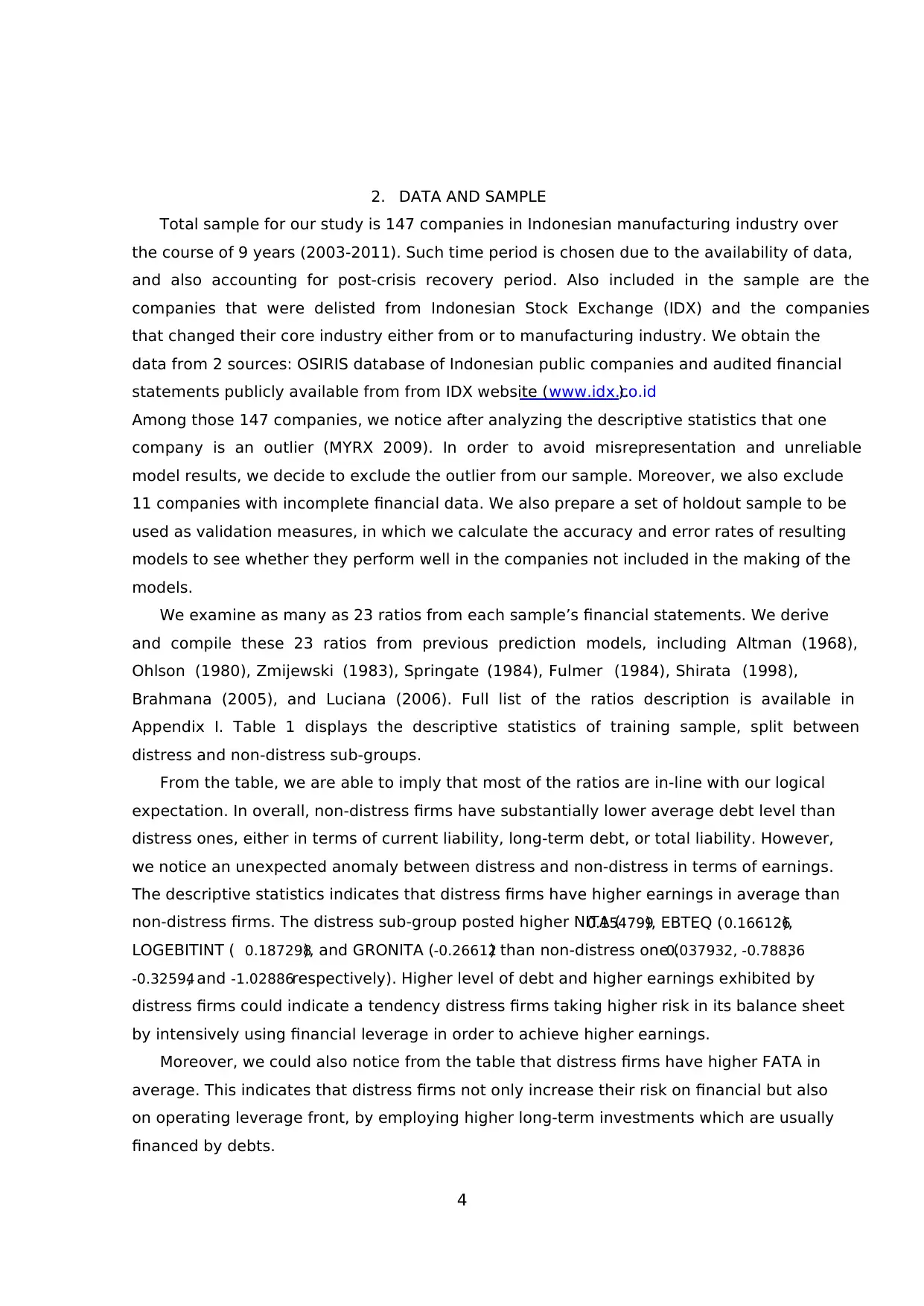
2. DATA AND SAMPLE
Total sample for our study is 147 companies in Indonesian manufacturing industry over
the course of 9 years (2003-2011). Such time period is chosen due to the availability of data,
and also accounting for post-crisis recovery period. Also included in the sample are the
companies that were delisted from Indonesian Stock Exchange (IDX) and the companies
that changed their core industry either from or to manufacturing industry. We obtain the
data from 2 sources: OSIRIS database of Indonesian public companies and audited financial
statements publicly available from from IDX website (www.idx.co.id).
Among those 147 companies, we notice after analyzing the descriptive statistics that one
company is an outlier (MYRX 2009). In order to avoid misrepresentation and unreliable
model results, we decide to exclude the outlier from our sample. Moreover, we also exclude
11 companies with incomplete financial data. We also prepare a set of holdout sample to be
used as validation measures, in which we calculate the accuracy and error rates of resulting
models to see whether they perform well in the companies not included in the making of the
models.
We examine as many as 23 ratios from each sample’s financial statements. We derive
and compile these 23 ratios from previous prediction models, including Altman (1968),
Ohlson (1980), Zmijewski (1983), Springate (1984), Fulmer (1984), Shirata (1998),
Brahmana (2005), and Luciana (2006). Full list of the ratios description is available in
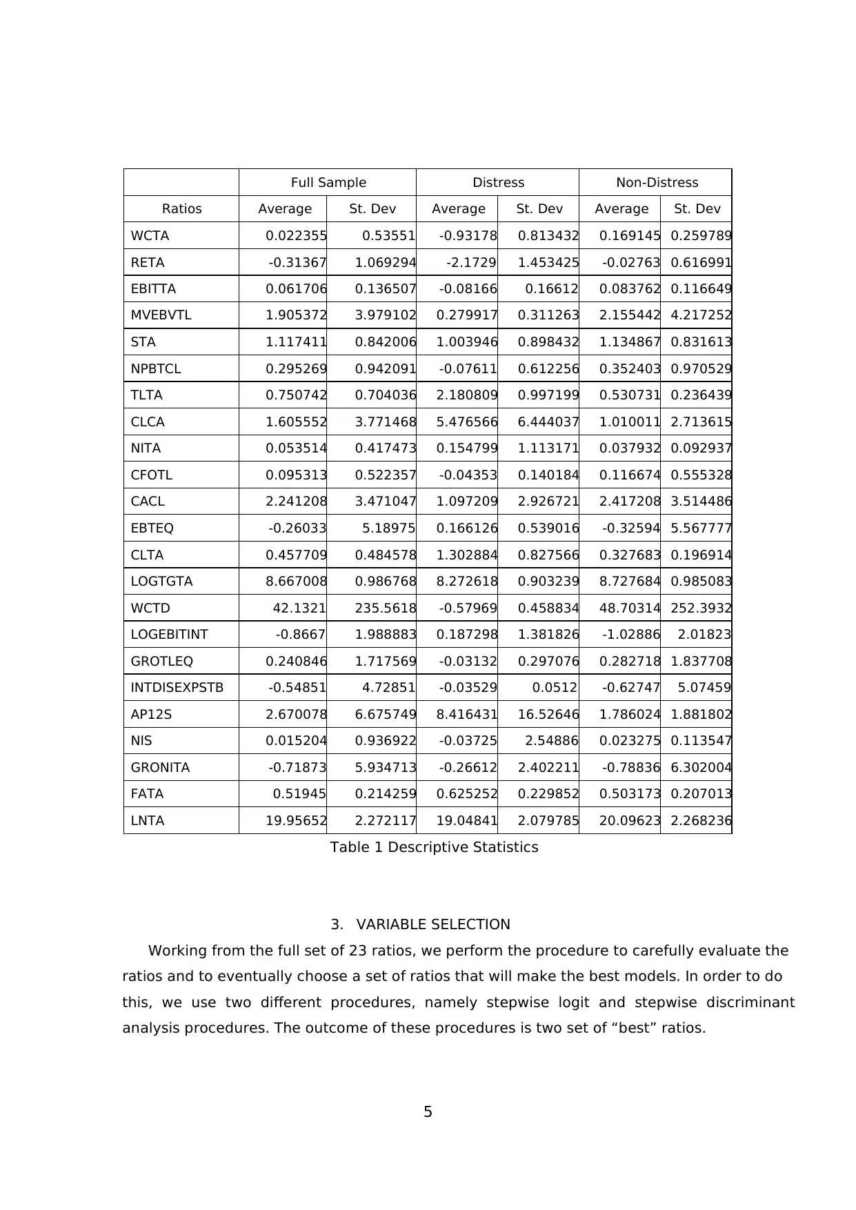
Appendix I. Table 1 displays the descriptive statistics of training sample, split between
distress and non-distress sub-groups.
From the table, we are able to imply that most of the ratios are in-line with our logical
expectation. In overall, non-distress firms have substantially lower average debt level than
distress ones, either in terms of current liability, long-term debt, or total liability. However,
we notice an unexpected anomaly between distress and non-distress in terms of earnings.
The descriptive statistics indicates that distress firms have higher earnings in average than
non-distress firms. The distress sub-group posted higher NITA (0.154799), EBTEQ (0.166126),
LOGEBITINT ( 0.187298), and GRONITA (-0.26612) than non-distress one (0.037932, -0.78836,
-0.32594, and -1.02886respectively). Higher level of debt and higher earnings exhibited by
distress firms could indicate a tendency distress firms taking higher risk in its balance sheet
by intensively using financial leverage in order to achieve higher earnings.
Moreover, we could also notice from the table that distress firms have higher FATA in
average. This indicates that distress firms not only increase their risk on financial but also
on operating leverage front, by employing higher long-term investments which are usually
financed by debts.
2. DATA AND SAMPLE
Total sample for our study is 147 companies in Indonesian manufacturing industry over
the course of 9 years (2003-2011). Such time period is chosen due to the availability of data,
and also accounting for post-crisis recovery period. Also included in the sample are the
companies that were delisted from Indonesian Stock Exchange (IDX) and the companies
that changed their core industry either from or to manufacturing industry. We obtain the
data from 2 sources: OSIRIS database of Indonesian public companies and audited financial
statements publicly available from from IDX website (www.idx.co.id).
Among those 147 companies, we notice after analyzing the descriptive statistics that one
company is an outlier (MYRX 2009). In order to avoid misrepresentation and unreliable
model results, we decide to exclude the outlier from our sample. Moreover, we also exclude
11 companies with incomplete financial data. We also prepare a set of holdout sample to be
used as validation measures, in which we calculate the accuracy and error rates of resulting
models to see whether they perform well in the companies not included in the making of the
models.
We examine as many as 23 ratios from each sample’s financial statements. We derive
and compile these 23 ratios from previous prediction models, including Altman (1968),
Ohlson (1980), Zmijewski (1983), Springate (1984), Fulmer (1984), Shirata (1998),
Brahmana (2005), and Luciana (2006). Full list of the ratios description is available in
Appendix I. Table 1 displays the descriptive statistics of training sample, split between
distress and non-distress sub-groups.
From the table, we are able to imply that most of the ratios are in-line with our logical
expectation. In overall, non-distress firms have substantially lower average debt level than
distress ones, either in terms of current liability, long-term debt, or total liability. However,
we notice an unexpected anomaly between distress and non-distress in terms of earnings.
The descriptive statistics indicates that distress firms have higher earnings in average than
non-distress firms. The distress sub-group posted higher NITA (0.154799), EBTEQ (0.166126),
LOGEBITINT ( 0.187298), and GRONITA (-0.26612) than non-distress one (0.037932, -0.78836,
-0.32594, and -1.02886respectively). Higher level of debt and higher earnings exhibited by
distress firms could indicate a tendency distress firms taking higher risk in its balance sheet
by intensively using financial leverage in order to achieve higher earnings.
Moreover, we could also notice from the table that distress firms have higher FATA in
average. This indicates that distress firms not only increase their risk on financial but also
on operating leverage front, by employing higher long-term investments which are usually
financed by debts.
5
Full Sample Distress Non-Distress
Ratios Average St. Dev Average St. Dev Average St. Dev
WCTA 0.022355 0.53551 -0.93178 0.813432 0.169145 0.259789
RETA -0.31367 1.069294 -2.1729 1.453425 -0.02763 0.616991
EBITTA 0.061706 0.136507 -0.08166 0.16612 0.083762 0.116649
MVEBVTL 1.905372 3.979102 0.279917 0.311263 2.155442 4.217252
STA 1.117411 0.842006 1.003946 0.898432 1.134867 0.831613
NPBTCL 0.295269 0.942091 -0.07611 0.612256 0.352403 0.970529
TLTA 0.750742 0.704036 2.180809 0.997199 0.530731 0.236439
CLCA 1.605552 3.771468 5.476566 6.444037 1.010011 2.713615
NITA 0.053514 0.417473 0.154799 1.113171 0.037932 0.092937
CFOTL 0.095313 0.522357 -0.04353 0.140184 0.116674 0.555328
CACL 2.241208 3.471047 1.097209 2.926721 2.417208 3.514486
EBTEQ -0.26033 5.18975 0.166126 0.539016 -0.32594 5.567777
CLTA 0.457709 0.484578 1.302884 0.827566 0.327683 0.196914
LOGTGTA 8.667008 0.986768 8.272618 0.903239 8.727684 0.985083
WCTD 42.1321 235.5618 -0.57969 0.458834 48.70314 252.3932
LOGEBITINT -0.8667 1.988883 0.187298 1.381826 -1.02886 2.01823
GROTLEQ 0.240846 1.717569 -0.03132 0.297076 0.282718 1.837708
INTDISEXPSTB -0.54851 4.72851 -0.03529 0.0512 -0.62747 5.07459
AP12S 2.670078 6.675749 8.416431 16.52646 1.786024 1.881802
NIS 0.015204 0.936922 -0.03725 2.54886 0.023275 0.113547
GRONITA -0.71873 5.934713 -0.26612 2.402211 -0.78836 6.302004
FATA 0.51945 0.214259 0.625252 0.229852 0.503173 0.207013
LNTA 19.95652 2.272117 19.04841 2.079785 20.09623 2.268236
Table 1 Descriptive Statistics
3. VARIABLE SELECTION
Working from the full set of 23 ratios, we perform the procedure to carefully evaluate the
ratios and to eventually choose a set of ratios that will make the best models. In order to do
this, we use two different procedures, namely stepwise logit and stepwise discriminant
analysis procedures. The outcome of these procedures is two set of “best” ratios.
⊘ This is a preview!⊘
Do you want full access?
Subscribe today to unlock all pages.
Trusted by 1+ million students worldwide
6
Stepwise Logit Procedure
For the first set of ratios, namely “Set I”, we utilize the stepwise logit method and
procedure as proposed by Draper and Smith (1981). We set the minimum level of
significance to enter the model at 0.05 and the maximum level of significance before removal
at 0.10. This means that a ratio must have a high significance value (p-value lower or at
most 0.05, note that the higher the significance, the lower the p-value) in order for us to
include the ratio into the Set I. After successfully included in the model, the ratio must
continuously score a high significance value when we repeat the procedure and enter other
ratios in order for it to stay in the Set I. If the ratio scores low significance value (p-value
higher than 0.10), we drop the ratio from the model. The procedure is stopped when any of
the previously entered ratios are excluded from the model due to having low significance.
Of all the ratios being analyzed, TLTA seems to have the biggest significance level, thus
we include ratio TLTA in Set I. The inclusion of TLTA somehow seems to damage the
reliability of our analysis, since it always dominates the significance level of the model
produced. TLTA also makes all other variables not significant. While this may be a sign that
TLTA is the only ratio we need to build a solid prediction model, as we go through model
estimation process, we eventually find that the prediction model with a single TLTA ratio
actually scores lower prediction power to other prediction models. Thus, we decide to exclude
TLTA from the beginning of the stepwise logit procedure.
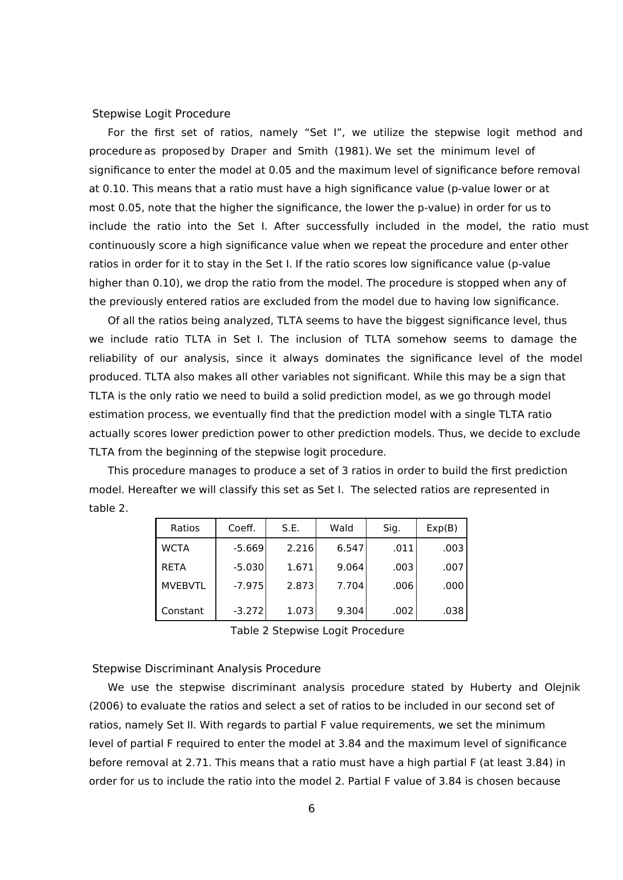
This procedure manages to produce a set of 3 ratios in order to build the first prediction
model. Hereafter we will classify this set as Set I. The selected ratios are represented in
table 2.
Ratios Coeff. S.E. Wald Sig. Exp(B)
WCTA -5.669 2.216 6.547 .011 .003
RETA -5.030 1.671 9.064 .003 .007
MVEBVTL -7.975 2.873 7.704 .006 .000
Constant -3.272 1.073 9.304 .002 .038
Table 2 Stepwise Logit Procedure
Stepwise Discriminant Analysis Procedure
We use the stepwise discriminant analysis procedure stated by Huberty and Olejnik
(2006) to evaluate the ratios and select a set of ratios to be included in our second set of
ratios, namely Set II. With regards to partial F value requirements, we set the minimum
level of partial F required to enter the model at 3.84 and the maximum level of significance
before removal at 2.71. This means that a ratio must have a high partial F (at least 3.84) in
order for us to include the ratio into the model 2. Partial F value of 3.84 is chosen because
Stepwise Logit Procedure
For the first set of ratios, namely “Set I”, we utilize the stepwise logit method and
procedure as proposed by Draper and Smith (1981). We set the minimum level of
significance to enter the model at 0.05 and the maximum level of significance before removal
at 0.10. This means that a ratio must have a high significance value (p-value lower or at
most 0.05, note that the higher the significance, the lower the p-value) in order for us to
include the ratio into the Set I. After successfully included in the model, the ratio must
continuously score a high significance value when we repeat the procedure and enter other
ratios in order for it to stay in the Set I. If the ratio scores low significance value (p-value
higher than 0.10), we drop the ratio from the model. The procedure is stopped when any of
the previously entered ratios are excluded from the model due to having low significance.
Of all the ratios being analyzed, TLTA seems to have the biggest significance level, thus
we include ratio TLTA in Set I. The inclusion of TLTA somehow seems to damage the
reliability of our analysis, since it always dominates the significance level of the model
produced. TLTA also makes all other variables not significant. While this may be a sign that
TLTA is the only ratio we need to build a solid prediction model, as we go through model
estimation process, we eventually find that the prediction model with a single TLTA ratio
actually scores lower prediction power to other prediction models. Thus, we decide to exclude
TLTA from the beginning of the stepwise logit procedure.
This procedure manages to produce a set of 3 ratios in order to build the first prediction
model. Hereafter we will classify this set as Set I. The selected ratios are represented in
table 2.
Ratios Coeff. S.E. Wald Sig. Exp(B)
WCTA -5.669 2.216 6.547 .011 .003
RETA -5.030 1.671 9.064 .003 .007
MVEBVTL -7.975 2.873 7.704 .006 .000
Constant -3.272 1.073 9.304 .002 .038
Table 2 Stepwise Logit Procedure
Stepwise Discriminant Analysis Procedure
We use the stepwise discriminant analysis procedure stated by Huberty and Olejnik
(2006) to evaluate the ratios and select a set of ratios to be included in our second set of
ratios, namely Set II. With regards to partial F value requirements, we set the minimum
level of partial F required to enter the model at 3.84 and the maximum level of significance
before removal at 2.71. This means that a ratio must have a high partial F (at least 3.84) in
order for us to include the ratio into the model 2. Partial F value of 3.84 is chosen because
Paraphrase This Document
Need a fresh take? Get an instant paraphrase of this document with our AI Paraphraser
7
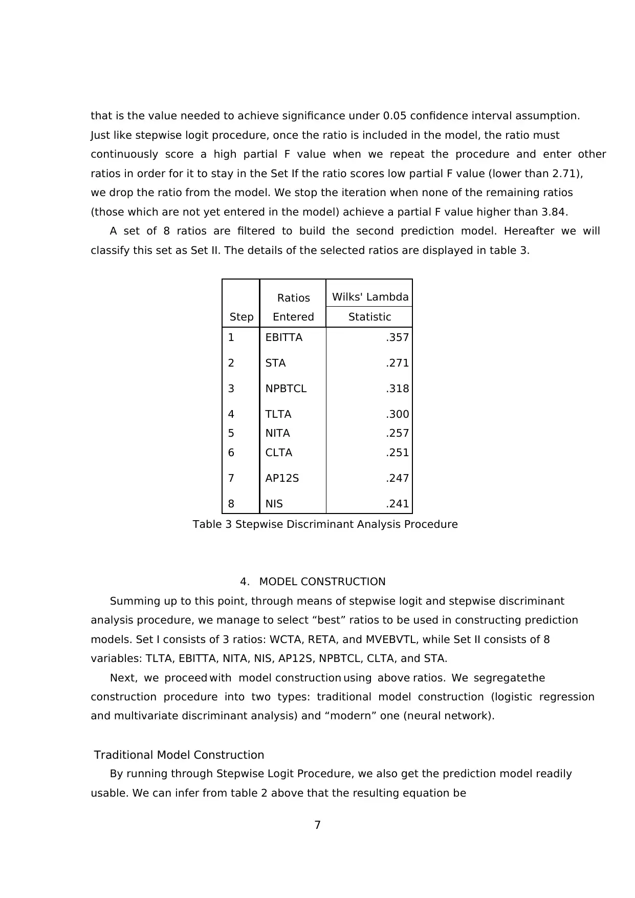
that is the value needed to achieve significance under 0.05 confidence interval assumption.
Just like stepwise logit procedure, once the ratio is included in the model, the ratio must
continuously score a high partial F value when we repeat the procedure and enter other
ratios in order for it to stay in the Set If the ratio scores low partial F value (lower than 2.71),
we drop the ratio from the model. We stop the iteration when none of the remaining ratios
(those which are not yet entered in the model) achieve a partial F value higher than 3.84.
A set of 8 ratios are filtered to build the second prediction model. Hereafter we will
classify this set as Set II. The details of the selected ratios are displayed in table 3.
Step
Ratios
Entered
Wilks' Lambda
Statistic
1 EBITTA .357
2 STA .271
3 NPBTCL .318
4 TLTA .300
5 NITA .257
6 CLTA .251
7 AP12S .247
8 NIS .241
Table 3 Stepwise Discriminant Analysis Procedure
4. MODEL CONSTRUCTION
Summing up to this point, through means of stepwise logit and stepwise discriminant
analysis procedure, we manage to select “best” ratios to be used in constructing prediction
models. Set I consists of 3 ratios: WCTA, RETA, and MVEBVTL, while Set II consists of 8
variables: TLTA, EBITTA, NITA, NIS, AP12S, NPBTCL, CLTA, and STA.
Next, we proceed with model construction using above ratios. We segregate the
construction procedure into two types: traditional model construction (logistic regression
and multivariate discriminant analysis) and “modern” one (neural network).
Traditional Model Construction
By running through Stepwise Logit Procedure, we also get the prediction model readily
usable. We can infer from table 2 above that the resulting equation be
8
1 ; where:
1 y
distress e −
= +
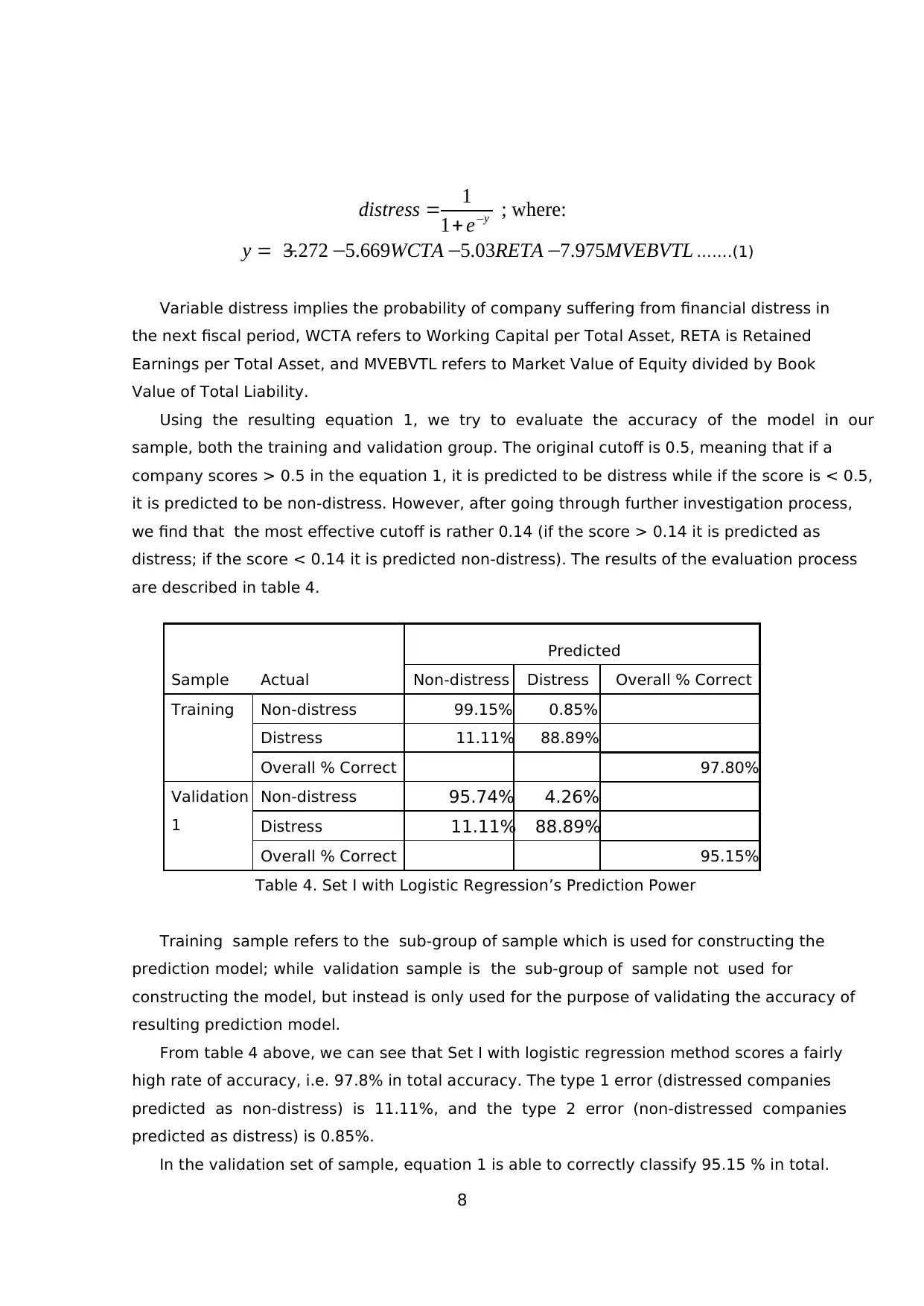
3.272 5.669 5.03 7.975y WCTA RETA MVEBVTL= − − − − …….(1)
Variable distress implies the probability of company suffering from financial distress in
the next fiscal period, WCTA refers to Working Capital per Total Asset, RETA is Retained
Earnings per Total Asset, and MVEBVTL refers to Market Value of Equity divided by Book
Value of Total Liability.
Using the resulting equation 1, we try to evaluate the accuracy of the model in our
sample, both the training and validation group. The original cutoff is 0.5, meaning that if a
company scores > 0.5 in the equation 1, it is predicted to be distress while if the score is < 0.5,
it is predicted to be non-distress. However, after going through further investigation process,
we find that the most effective cutoff is rather 0.14 (if the score > 0.14 it is predicted as
distress; if the score < 0.14 it is predicted non-distress). The results of the evaluation process
are described in table 4.
Sample Actual
Predicted
Non-distress Distress Overall % Correct
Training Non-distress 99.15% 0.85%
Distress 11.11% 88.89%
Overall % Correct 97.80%
Validation
1
Non-distress 95.74% 4.26%
Distress 11.11% 88.89%
Overall % Correct 95.15%
Table 4. Set I with Logistic Regression’s Prediction Power
Training sample refers to the sub-group of sample which is used for constructing the
prediction model; while validation sample is the sub-group of sample not used for
constructing the model, but instead is only used for the purpose of validating the accuracy of
resulting prediction model.
From table 4 above, we can see that Set I with logistic regression method scores a fairly
high rate of accuracy, i.e. 97.8% in total accuracy. The type 1 error (distressed companies
predicted as non-distress) is 11.11%, and the type 2 error (non-distressed companies
predicted as distress) is 0.85%.
In the validation set of sample, equation 1 is able to correctly classify 95.15 % in total.
1 ; where:
1 y
distress e −
= +
3.272 5.669 5.03 7.975y WCTA RETA MVEBVTL= − − − − …….(1)
Variable distress implies the probability of company suffering from financial distress in
the next fiscal period, WCTA refers to Working Capital per Total Asset, RETA is Retained
Earnings per Total Asset, and MVEBVTL refers to Market Value of Equity divided by Book
Value of Total Liability.
Using the resulting equation 1, we try to evaluate the accuracy of the model in our
sample, both the training and validation group. The original cutoff is 0.5, meaning that if a
company scores > 0.5 in the equation 1, it is predicted to be distress while if the score is < 0.5,
it is predicted to be non-distress. However, after going through further investigation process,
we find that the most effective cutoff is rather 0.14 (if the score > 0.14 it is predicted as
distress; if the score < 0.14 it is predicted non-distress). The results of the evaluation process
are described in table 4.
Sample Actual
Predicted
Non-distress Distress Overall % Correct
Training Non-distress 99.15% 0.85%
Distress 11.11% 88.89%
Overall % Correct 97.80%
Validation
1
Non-distress 95.74% 4.26%
Distress 11.11% 88.89%
Overall % Correct 95.15%
Table 4. Set I with Logistic Regression’s Prediction Power
Training sample refers to the sub-group of sample which is used for constructing the
prediction model; while validation sample is the sub-group of sample not used for
constructing the model, but instead is only used for the purpose of validating the accuracy of
resulting prediction model.
From table 4 above, we can see that Set I with logistic regression method scores a fairly
high rate of accuracy, i.e. 97.8% in total accuracy. The type 1 error (distressed companies
predicted as non-distress) is 11.11%, and the type 2 error (non-distressed companies
predicted as distress) is 0.85%.
In the validation set of sample, equation 1 is able to correctly classify 95.15 % in total.
⊘ This is a preview!⊘
Do you want full access?
Subscribe today to unlock all pages.
Trusted by 1+ million students worldwide
9
The characteristic of error is also quite acceptable, with type 1 error at 11.11% and type 2
error at 4.26%.
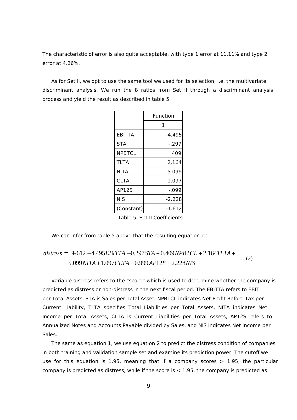
As for Set II, we opt to use the same tool we used for its selection, i.e. the multivariate
discriminant analysis. We run the 8 ratios from Set II through a discriminant analysis
process and yield the result as described in table 5.
Function
1
EBITTA -4.495
STA -.297
NPBTCL .409
TLTA 2.164
NITA 5.099
CLTA 1.097
AP12S -.099
NIS -2.228
(Constant) -1.612
Table 5. Set II Coefficients
We can infer from table 5 above that the resulting equation be
1.612 4.495 0.297 0.409 2.164
5.099 1.097 0.999 12 2.228
distress EBITTA STA NPBTCL TLTA
NITA CLTA AP S NIS
= − − − + + +
+ − − ….(2)
Variable distress refers to the “score” which is used to determine whether the company is
predicted as distress or non-distress in the next fiscal period. The EBITTA refers to EBIT
per Total Assets, STA is Sales per Total Asset, NPBTCL indicates Net Profit Before Tax per
Current Liability, TLTA specifies Total Liabilities per Total Assets, NITA indicates Net
Income per Total Assets, CLTA is Current Liabilities per Total Assets, AP12S refers to
Annualized Notes and Accounts Payable divided by Sales, and NIS indicates Net Income per
Sales.
The same as equation 1, we use equation 2 to predict the distress condition of companies
in both training and validation sample set and examine its prediction power. The cutoff we
use for this equation is 1.95, meaning that if a company scores > 1.95, the particular
company is predicted as distress, while if the score is < 1.95, the company is predicted as
The characteristic of error is also quite acceptable, with type 1 error at 11.11% and type 2
error at 4.26%.
As for Set II, we opt to use the same tool we used for its selection, i.e. the multivariate
discriminant analysis. We run the 8 ratios from Set II through a discriminant analysis
process and yield the result as described in table 5.
Function
1
EBITTA -4.495
STA -.297
NPBTCL .409
TLTA 2.164
NITA 5.099
CLTA 1.097
AP12S -.099
NIS -2.228
(Constant) -1.612
Table 5. Set II Coefficients
We can infer from table 5 above that the resulting equation be
1.612 4.495 0.297 0.409 2.164
5.099 1.097 0.999 12 2.228
distress EBITTA STA NPBTCL TLTA
NITA CLTA AP S NIS
= − − − + + +
+ − − ….(2)
Variable distress refers to the “score” which is used to determine whether the company is
predicted as distress or non-distress in the next fiscal period. The EBITTA refers to EBIT
per Total Assets, STA is Sales per Total Asset, NPBTCL indicates Net Profit Before Tax per
Current Liability, TLTA specifies Total Liabilities per Total Assets, NITA indicates Net
Income per Total Assets, CLTA is Current Liabilities per Total Assets, AP12S refers to
Annualized Notes and Accounts Payable divided by Sales, and NIS indicates Net Income per
Sales.
The same as equation 1, we use equation 2 to predict the distress condition of companies
in both training and validation sample set and examine its prediction power. The cutoff we
use for this equation is 1.95, meaning that if a company scores > 1.95, the particular
company is predicted as distress, while if the score is < 1.95, the company is predicted as
Paraphrase This Document
Need a fresh take? Get an instant paraphrase of this document with our AI Paraphraser
10
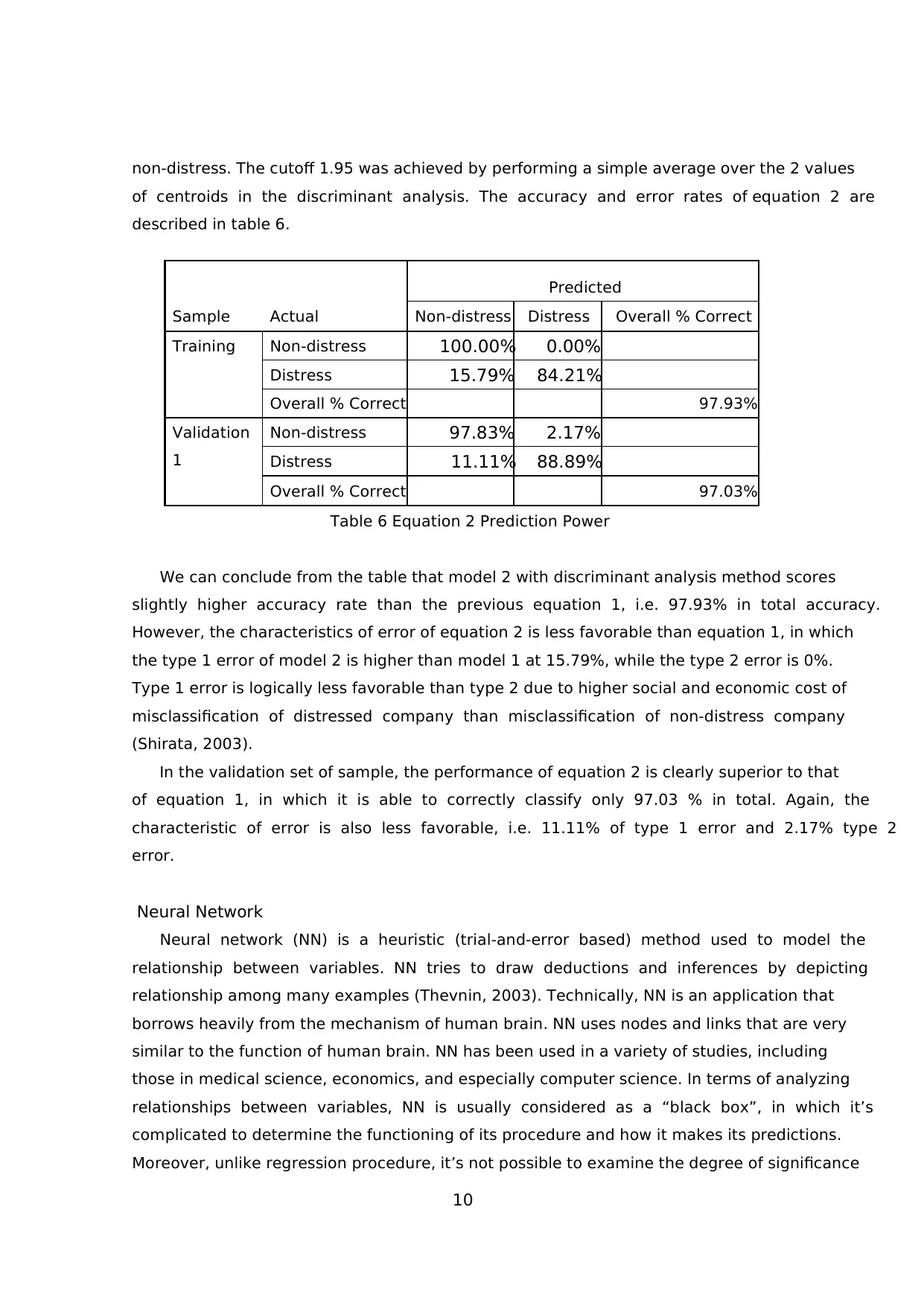
non-distress. The cutoff 1.95 was achieved by performing a simple average over the 2 values
of centroids in the discriminant analysis. The accuracy and error rates of equation 2 are
described in table 6.
Sample Actual
Predicted
Non-distress Distress Overall % Correct
Training Non-distress 100.00% 0.00%
Distress 15.79% 84.21%
Overall % Correct 97.93%
Validation
1
Non-distress 97.83% 2.17%
Distress 11.11% 88.89%
Overall % Correct 97.03%
Table 6 Equation 2 Prediction Power
We can conclude from the table that model 2 with discriminant analysis method scores
slightly higher accuracy rate than the previous equation 1, i.e. 97.93% in total accuracy.
However, the characteristics of error of equation 2 is less favorable than equation 1, in which
the type 1 error of model 2 is higher than model 1 at 15.79%, while the type 2 error is 0%.
Type 1 error is logically less favorable than type 2 due to higher social and economic cost of
misclassification of distressed company than misclassification of non-distress company
(Shirata, 2003).
In the validation set of sample, the performance of equation 2 is clearly superior to that
of equation 1, in which it is able to correctly classify only 97.03 % in total. Again, the
characteristic of error is also less favorable, i.e. 11.11% of type 1 error and 2.17% type 2
error.
Neural Network
Neural network (NN) is a heuristic (trial-and-error based) method used to model the
relationship between variables. NN tries to draw deductions and inferences by depicting
relationship among many examples (Thevnin, 2003). Technically, NN is an application that
borrows heavily from the mechanism of human brain. NN uses nodes and links that are very
similar to the function of human brain. NN has been used in a variety of studies, including
those in medical science, economics, and especially computer science. In terms of analyzing
relationships between variables, NN is usually considered as a “black box”, in which it’s
complicated to determine the functioning of its procedure and how it makes its predictions.
Moreover, unlike regression procedure, it’s not possible to examine the degree of significance
11
of each independent variable. Another major weakness of NN is that it is considerably more
complicated to use compared to a simple and ready-to-use equation produced by logistic
regression or discriminant analysis procedure. Thus a proven and good-performing NN
model might not be able to be exactly replicated by other researchers (for academic purpose)
or to be applied in practice by the common investor. However, unlike traditional statistical
tools which are incapable of identifying non-linear relationship, NN is able to identify either
linear or non-linear relationship that exists in the dataset (Khajanchi, 2002), thus making it
a relatively more powerful predictor than traditional statistical tools.
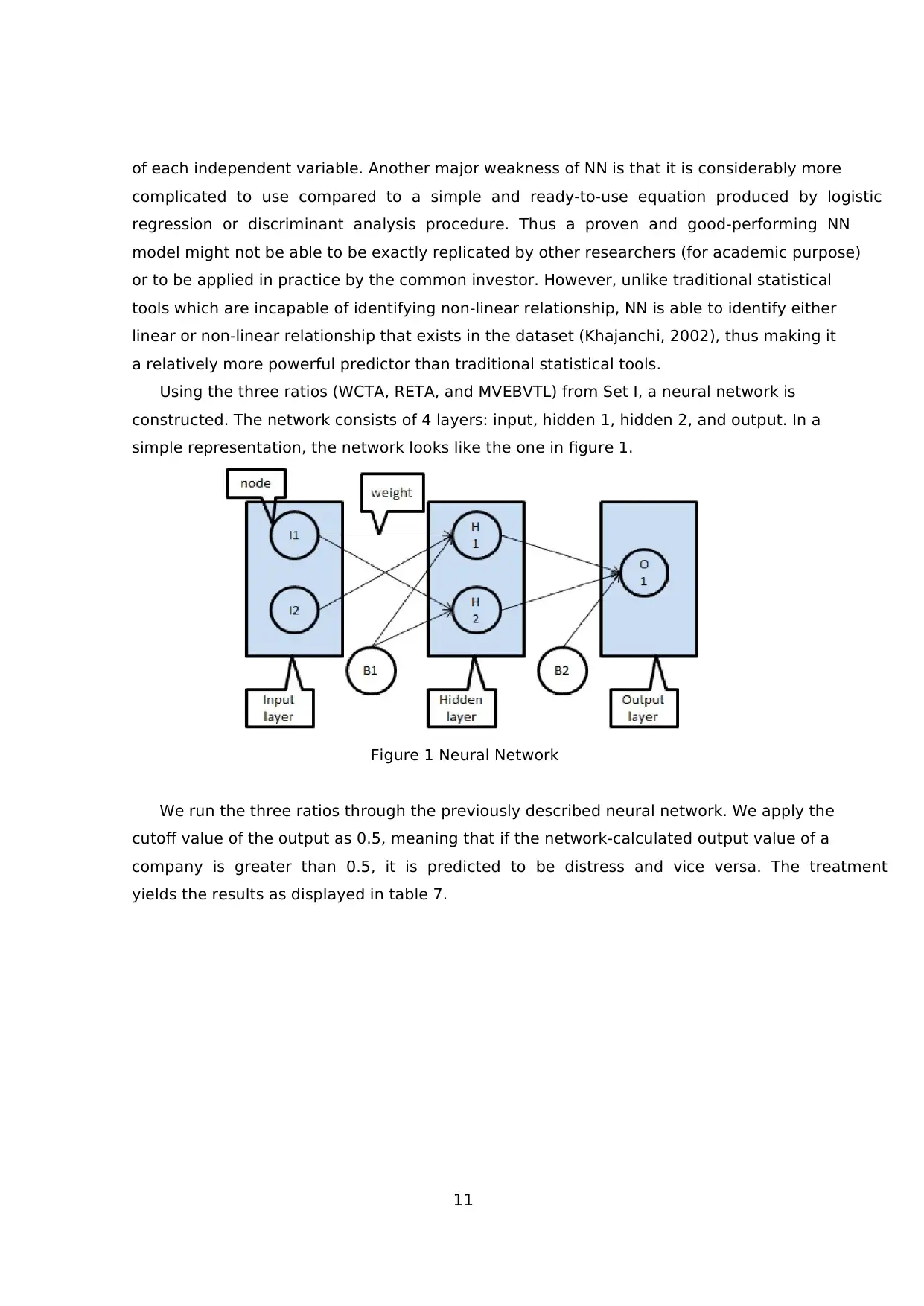
Using the three ratios (WCTA, RETA, and MVEBVTL) from Set I, a neural network is
constructed. The network consists of 4 layers: input, hidden 1, hidden 2, and output. In a
simple representation, the network looks like the one in figure 1.
Figure 1 Neural Network
We run the three ratios through the previously described neural network. We apply the
cutoff value of the output as 0.5, meaning that if the network-calculated output value of a
company is greater than 0.5, it is predicted to be distress and vice versa. The treatment
yields the results as displayed in table 7.
of each independent variable. Another major weakness of NN is that it is considerably more
complicated to use compared to a simple and ready-to-use equation produced by logistic
regression or discriminant analysis procedure. Thus a proven and good-performing NN
model might not be able to be exactly replicated by other researchers (for academic purpose)
or to be applied in practice by the common investor. However, unlike traditional statistical
tools which are incapable of identifying non-linear relationship, NN is able to identify either
linear or non-linear relationship that exists in the dataset (Khajanchi, 2002), thus making it
a relatively more powerful predictor than traditional statistical tools.
Using the three ratios (WCTA, RETA, and MVEBVTL) from Set I, a neural network is
constructed. The network consists of 4 layers: input, hidden 1, hidden 2, and output. In a
simple representation, the network looks like the one in figure 1.
Figure 1 Neural Network
We run the three ratios through the previously described neural network. We apply the
cutoff value of the output as 0.5, meaning that if the network-calculated output value of a
company is greater than 0.5, it is predicted to be distress and vice versa. The treatment
yields the results as displayed in table 7.
⊘ This is a preview!⊘
Do you want full access?
Subscribe today to unlock all pages.
Trusted by 1+ million students worldwide
1 out of 22


Your All-in-One AI-Powered Toolkit for Academic Success.
+13062052269
info@desklib.com
Available 24*7 on WhatsApp / Email
![[object Object]](/_next/static/media/star-bottom.7253800d.svg)
Unlock your academic potential
Copyright © 2020–2026 A2Z Services. All Rights Reserved. Developed and managed by ZUCOL.