ME504 Industrial Instrumentation Assessment: Temperature Step Response

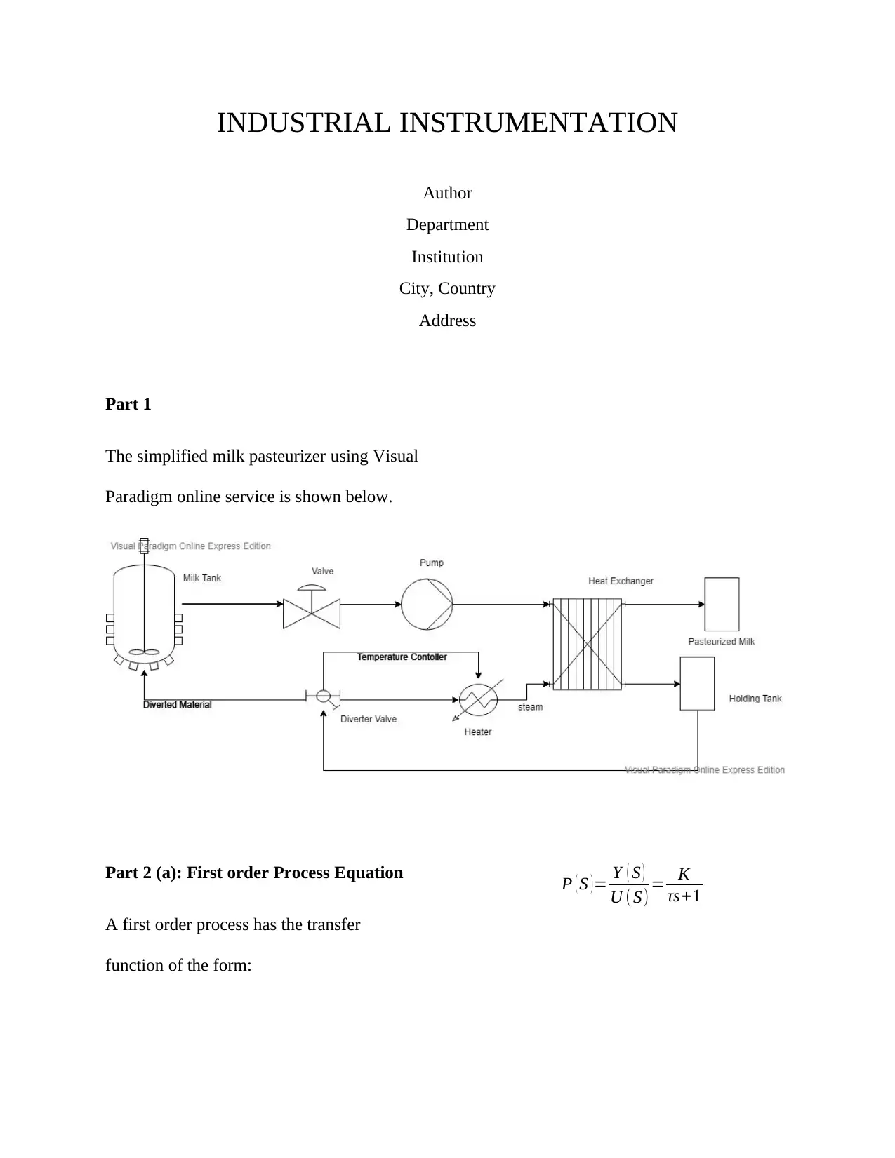
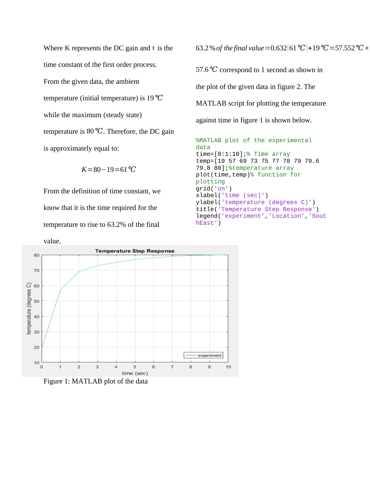
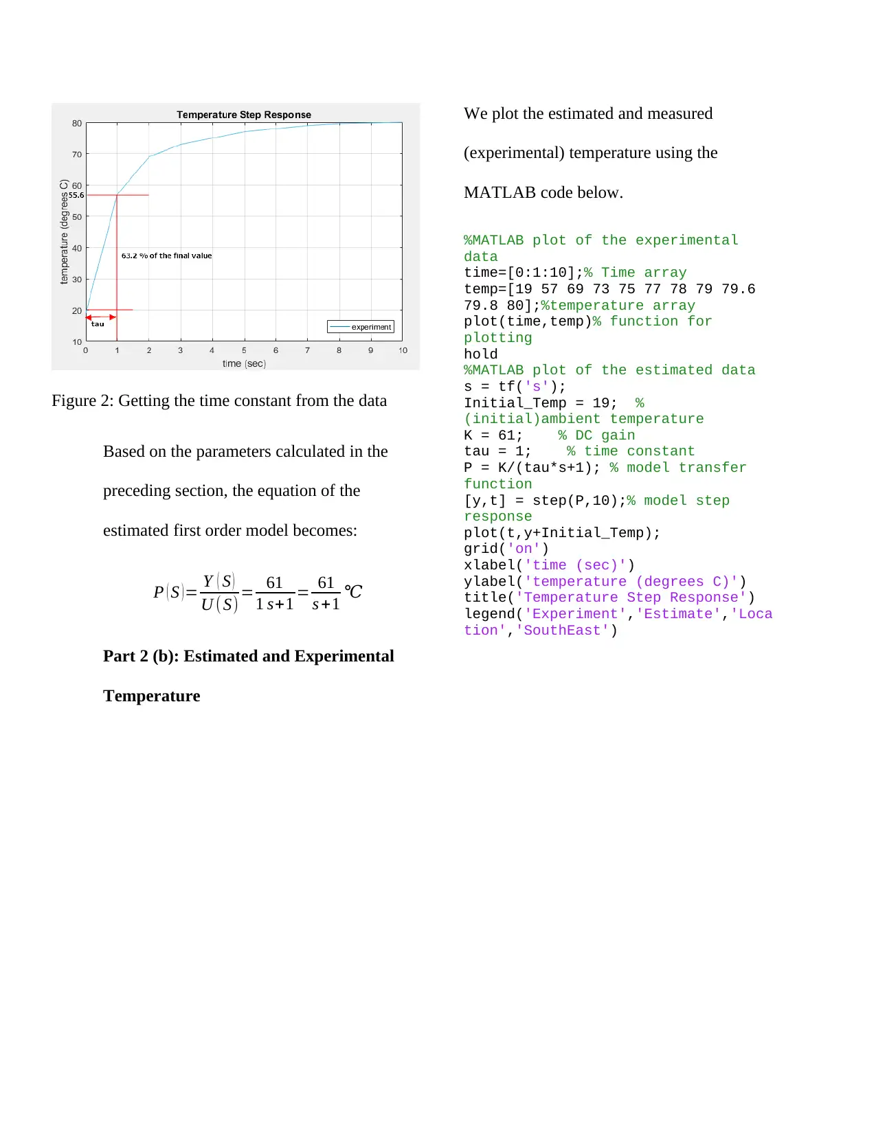
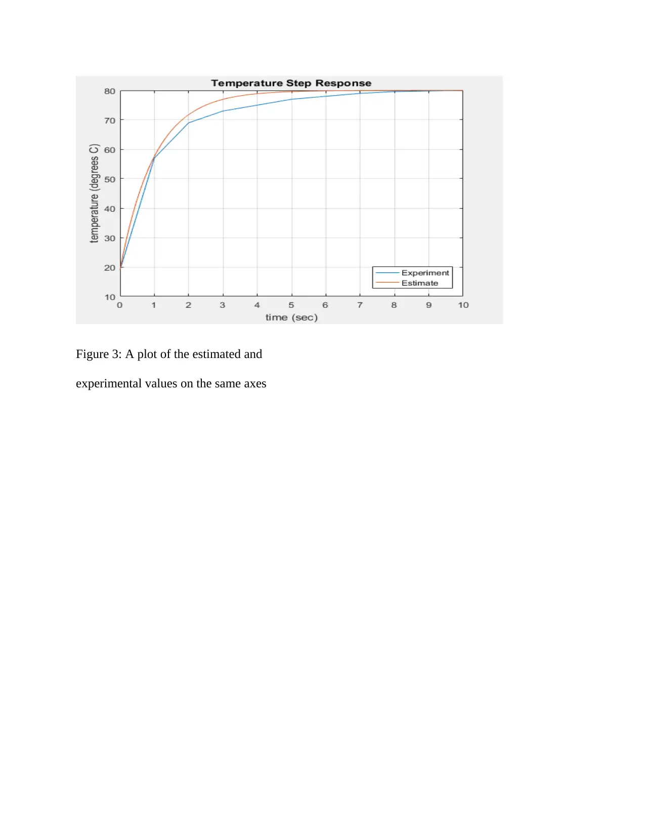
This assignment focuses on the analysis and modeling of a milk pasteurizer's temperature step response. It begins with a simplified model of the pasteurizer and proceeds to derive the first-order process equation, calculating the DC gain and time constant from given data. The solution utilizes MATLAB to plot the experimental data and estimate the model parameters. The assignment then compares the estimated and experimental temperature values using MATLAB, providing plots and code for both. The document demonstrates the application of control system principles to analyze and model a real-world industrial process, offering a practical example of system identification and process control techniques in industrial automation.

INDUSTRIAL INSTRUMENTATION
Author
Department
Institution
City, Country
Address
Part 1
The simplified milk pasteurizer using Visual
Paradigm online service is shown below.
Part 2 (a): First order Process Equation
A first order process has the transfer
function of the form:
P ( S ) = Y ( S )
U ( S) = K
τs+1

Where K represents the DC gain and τ is the
time constant of the first order process.
From the given data, the ambient
temperature (initial temperature) is 19 ℃
while the maximum (steady state)
temperature is 80 ℃. Therefore, the DC gain
is approximately equal to:
K=80−19=61℃
From the definition of time constant, we
know that it is the time required for the
temperature to rise to 63.2% of the final
value.
63.2 % of the final value=0.632 ( 61 ℃ ) +19 ℃=57.552℃ ≅ 5
57.6 ℃ correspond to 1 second as shown in
the plot of the given data in figure 2. The
MATLAB script for plotting the temperature
against time in figure 1 is shown below.
%MATLAB plot of the experimental
data
time=[0:1:10];% Time array
temp=[19 57 69 73 75 77 78 79 79.6
79.8 80];%temperature array
plot(time,temp)% function for
plotting
grid('on')
xlabel('time (sec)')
ylabel('temperature (degrees C)')
title('Temperature Step Response')
legend('experiment','Location','Sout
hEast')
Figure 1: MATLAB plot of the data

Figure 2: Getting the time constant from the data
Based on the parameters calculated in the
preceding section, the equation of the
estimated first order model becomes:
P ( S ) = Y ( S )
U ( S) = 61
1 s+1 = 61
s +1 ℃
Part 2 (b): Estimated and Experimental
Temperature
We plot the estimated and measured
(experimental) temperature using the
MATLAB code below.
%MATLAB plot of the experimental
data
time=[0:1:10];% Time array
temp=[19 57 69 73 75 77 78 79 79.6
79.8 80];%temperature array
plot(time,temp)% function for
plotting
hold
%MATLAB plot of the estimated data
s = tf('s');
Initial_Temp = 19; %
(initial)ambient temperature
K = 61; % DC gain
tau = 1; % time constant
P = K/(tau*s+1); % model transfer
function
[y,t] = step(P,10);% model step
response
plot(t,y+Initial_Temp);
grid('on')
xlabel('time (sec)')
ylabel('temperature (degrees C)')
title('Temperature Step Response')
legend('Experiment','Estimate','Loca
tion','SouthEast')

Figure 3: A plot of the estimated and
experimental values on the same axes