ME503 Industrial Process Control Systems: PID Controller Design Report
VerifiedAdded on 2023/06/03
|28
|5000
|119
Report
AI Summary
This report focuses on the design and simulation of a PID controller for industrial process control systems. It begins with an overview of industrial automation and the role of PID controllers in maintaining process enactment. The report outlines the aims and objectives, including system design using MATLAB and the application of the Cohen-Coon tuning method to a mixer system. It details the design methodology, covering process, control valve, and transport lag transfer functions, along with key control variables like steady-state error, rise time, overshoot, and system stability. The report explores various loop tuning methods, including manual tuning, Ziegler-Nichols, and Cohen-Coon, before delving into the design, simulation, and MATLAB implementation of the PID controller. Results and observations are presented, followed by a discussion on the flexibility, availability, and cost-effectiveness of using PLCs for implementation, as well as considerations for safety-critical shutdown systems.
Paraphrase This Document
Need a fresh take? Get an instant paraphrase of this document with our AI Paraphraser
TABLE OF CONTENTS
1. INTRODUCTION...............................................................................................................................2
Basic Overview.......................................................................................................................................2
2. AIMS AND OBJECTIVES.................................................................................................................7
3. PROBLEM STATEMENT..................................................................................................................7
4. DESIGN METHODOLOGY...............................................................................................................7
5. LOOP TUNING METHODS............................................................................................................11
Manual tuning Method..........................................................................................................................12
Ziegler-Nichols method.........................................................................................................................12
Cohen-Coon Method.............................................................................................................................14
6. DESIGN, SIMULATION AND MATLAB IMPLEMENTATION...................................................16
7. RESULTS AND OBSERVATION...................................................................................................18
8. DISCUSSION...................................................................................................................................21
PLC for implementation- flexibility, availability, and cost....................................................................22
Safety critical shutdown system............................................................................................................24
REFERENCES..........................................................................................................................................26
2
1. INTRODUCTION
Basic Overview
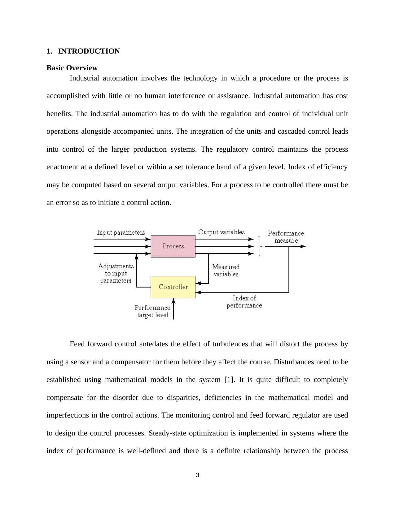
Industrial automation involves the technology in which a procedure or the process is
accomplished with little or no human interference or assistance. Industrial automation has cost
benefits. The industrial automation has to do with the regulation and control of individual unit
operations alongside accompanied units. The integration of the units and cascaded control leads
into control of the larger production systems. The regulatory control maintains the process
enactment at a defined level or within a set tolerance band of a given level. Index of efficiency
may be computed based on several output variables. For a process to be controlled there must be
an error so as to initiate a control action.
Feed forward control antedates the effect of turbulences that will distort the process by
using a sensor and a compensator for them before they affect the course. Disturbances need to be
established using mathematical models in the system [1]. It is quite difficult to completely
compensate for the disorder due to disparities, deficiencies in the mathematical model and
imperfections in the control actions. The monitoring control and feed forward regulator are used
to design the control processes. Steady-state optimization is implemented in systems where the
index of performance is well-defined and there is a definite relationship between the process
3
Basic Overview
Industrial automation involves the technology in which a procedure or the process is
accomplished with little or no human interference or assistance. Industrial automation has cost
benefits. The industrial automation has to do with the regulation and control of individual unit
operations alongside accompanied units. The integration of the units and cascaded control leads
into control of the larger production systems. The regulatory control maintains the process
enactment at a defined level or within a set tolerance band of a given level. Index of efficiency
may be computed based on several output variables. For a process to be controlled there must be
an error so as to initiate a control action.
Feed forward control antedates the effect of turbulences that will distort the process by
using a sensor and a compensator for them before they affect the course. Disturbances need to be
established using mathematical models in the system [1]. It is quite difficult to completely
compensate for the disorder due to disparities, deficiencies in the mathematical model and
imperfections in the control actions. The monitoring control and feed forward regulator are used
to design the control processes. Steady-state optimization is implemented in systems where the
index of performance is well-defined and there is a definite relationship between the process
3
⊘ This is a preview!⊘
Do you want full access?
Subscribe today to unlock all pages.
Trusted by 1+ million students worldwide
variables and IP. Mathematical models are used to optimize the index of performance based on
system parameter values.
The most commonly used controller in industrial applications is the proportional-integral-
derivative controller. The PID controller computes the error value which results from the
alteration between the anticipated output or yield and the measured process variable. A feedback
loop is used to perform the computation. The feedback loop mainly contains a sensor which
collects data from the output and relays it to the error computation point. The controller has three
segments namely the proportional, the integral, the derivative. The proportional term relies on
the current errors, the integral component relies on the accumulation of the past errors, and the
derivative component relies on the prediction of the future errors. The impact of these three
components brings about change when implemented in the regulating valve before the mixing
process commences. It is quite a crucial component in industrial implementations and the
controller can deliver control action intended for specific process requirements [2].
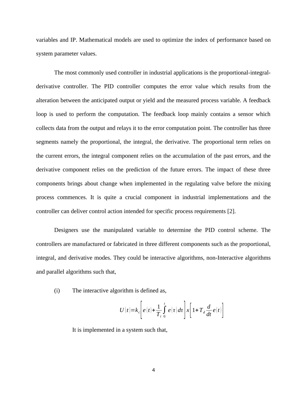
Designers use the manipulated variable to determine the PID control scheme. The
controllers are manufactured or fabricated in three different components such as the proportional,
integral, and derivative modes. They could be interactive algorithms, non-Interactive algorithms
and parallel algorithms such that,
(i) The interactive algorithm is defined as,
U ( t ) =kc [ e ( t ) + 1
Ti
∫
0
t
e ( τ ) dτ ] x [ 1+ Td
d
dt e ( t ) ]
It is implemented in a system such that,
4
system parameter values.
The most commonly used controller in industrial applications is the proportional-integral-
derivative controller. The PID controller computes the error value which results from the
alteration between the anticipated output or yield and the measured process variable. A feedback
loop is used to perform the computation. The feedback loop mainly contains a sensor which
collects data from the output and relays it to the error computation point. The controller has three
segments namely the proportional, the integral, the derivative. The proportional term relies on
the current errors, the integral component relies on the accumulation of the past errors, and the
derivative component relies on the prediction of the future errors. The impact of these three
components brings about change when implemented in the regulating valve before the mixing
process commences. It is quite a crucial component in industrial implementations and the
controller can deliver control action intended for specific process requirements [2].
Designers use the manipulated variable to determine the PID control scheme. The
controllers are manufactured or fabricated in three different components such as the proportional,
integral, and derivative modes. They could be interactive algorithms, non-Interactive algorithms
and parallel algorithms such that,
(i) The interactive algorithm is defined as,
U ( t ) =kc [ e ( t ) + 1
Ti
∫
0
t
e ( τ ) dτ ] x [ 1+ Td
d
dt e ( t ) ]
It is implemented in a system such that,
4
Paraphrase This Document
Need a fresh take? Get an instant paraphrase of this document with our AI Paraphraser
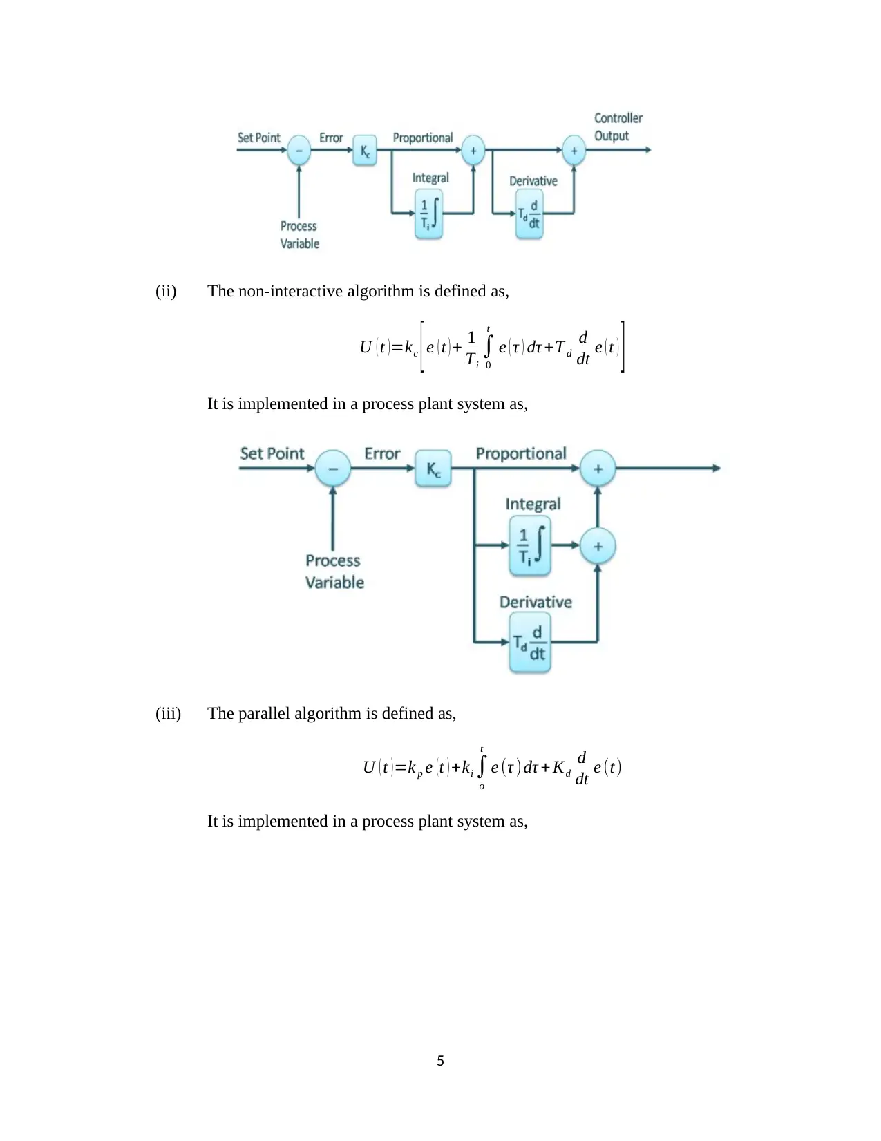
(ii) The non-interactive algorithm is defined as,
U ( t )=kc [e ( t ) + 1
Ti
∫
0
t
e ( τ ) dτ +T d
d
dt e ( t ) ]
It is implemented in a process plant system as,
(iii) The parallel algorithm is defined as,
U ( t )=k p e (t ) +ki ∫
o
t
e (τ )dτ + Kd
d
dt e (t)
It is implemented in a process plant system as,
5
U ( t )=kc [e ( t ) + 1
Ti
∫
0
t
e ( τ ) dτ +T d
d
dt e ( t ) ]
It is implemented in a process plant system as,
(iii) The parallel algorithm is defined as,
U ( t )=k p e (t ) +ki ∫
o
t
e (τ )dτ + Kd
d
dt e (t)
It is implemented in a process plant system as,
5
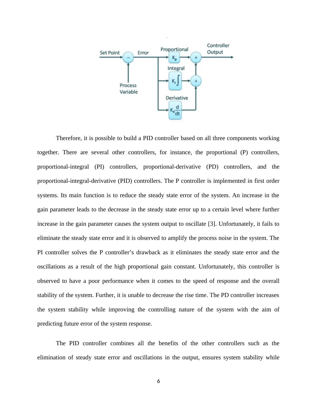
Therefore, it is possible to build a PID controller based on all three components working
together. There are several other controllers, for instance, the proportional (P) controllers,
proportional-integral (PI) controllers, proportional-derivative (PD) controllers, and the
proportional-integral-derivative (PID) controllers. The P controller is implemented in first order
systems. Its main function is to reduce the steady state error of the system. An increase in the
gain parameter leads to the decrease in the steady state error up to a certain level where further
increase in the gain parameter causes the system output to oscillate [3]. Unfortunately, it fails to
eliminate the steady state error and it is observed to amplify the process noise in the system. The
PI controller solves the P controller’s drawback as it eliminates the steady state error and the
oscillations as a result of the high proportional gain constant. Unfortunately, this controller is
observed to have a poor performance when it comes to the speed of response and the overall
stability of the system. Further, it is unable to decrease the rise time. The PD controller increases
the system stability while improving the controlling nature of the system with the aim of
predicting future error of the system response.
The PID controller combines all the benefits of the other controllers such as the
elimination of steady state error and oscillations in the output, ensures system stability while
6
⊘ This is a preview!⊘
Do you want full access?
Subscribe today to unlock all pages.
Trusted by 1+ million students worldwide
controlling the process plant, as well as decreasing the rise time. The controller can be used with
single energy systems or the commonly known first order systems as well as with higher order
systems.
It is perceived that, when the step response of the system is obtained, the output response
is given as,
(i) Increasing the proportional constant reduces the steady state error.
(ii) Increasing the proportional constant after a given value may cause an overshoot.
(iii) Increasing the proportional constant may reduce the rise time.
(iv) The integral control eliminates the steady state error.
(v) The limit increases the integral constant and increases the overshoot.
(vi) Slightly increasing the integral constant reduces the rise time by a small value.
(vii) Increasing the derivative constant decreases the overshoot.
(viii) Increasing the derivative constant reduces the settling time.
A feedback loop may undergo tuning so as to ensure that all the control strictures are
implemented to their optimum principles so as to obtain the preferred control response.
Controller tuning requires that one chooses a good initial set of controller parameter values to
avoid leading the system to instability or cause it to have a deterioration of performance of the
closed loop system. Tuning seeks to find the optimum settings of the PID parameters such as the
proportional constant, integral constant, and the derivative constant through experimentation or
following specific tuning methods. The process of tuning can be done for both open loop and
closed loop systems. The output is expected to be steady and it should not waver at any condition
of the set point or disturbance. The bounded oscillation condition for a marginal stability is
accepted. The process is expected to meet the regulation and command breaking requirements as
set by the controller designer. To meet the command breaking requirements, the designer
7
Paraphrase This Document
Need a fresh take? Get an instant paraphrase of this document with our AI Paraphraser
focused on the rise time and settling time attributes of a system response. The system controller
in section 5 discusses the methods used in tuning a control loop.
2. AIMS AND OBJECTIVES
(i) To determine the system design using MATLAB software
(ii) To design the mixer system with a PID controller and Cohen-coon tuning method.
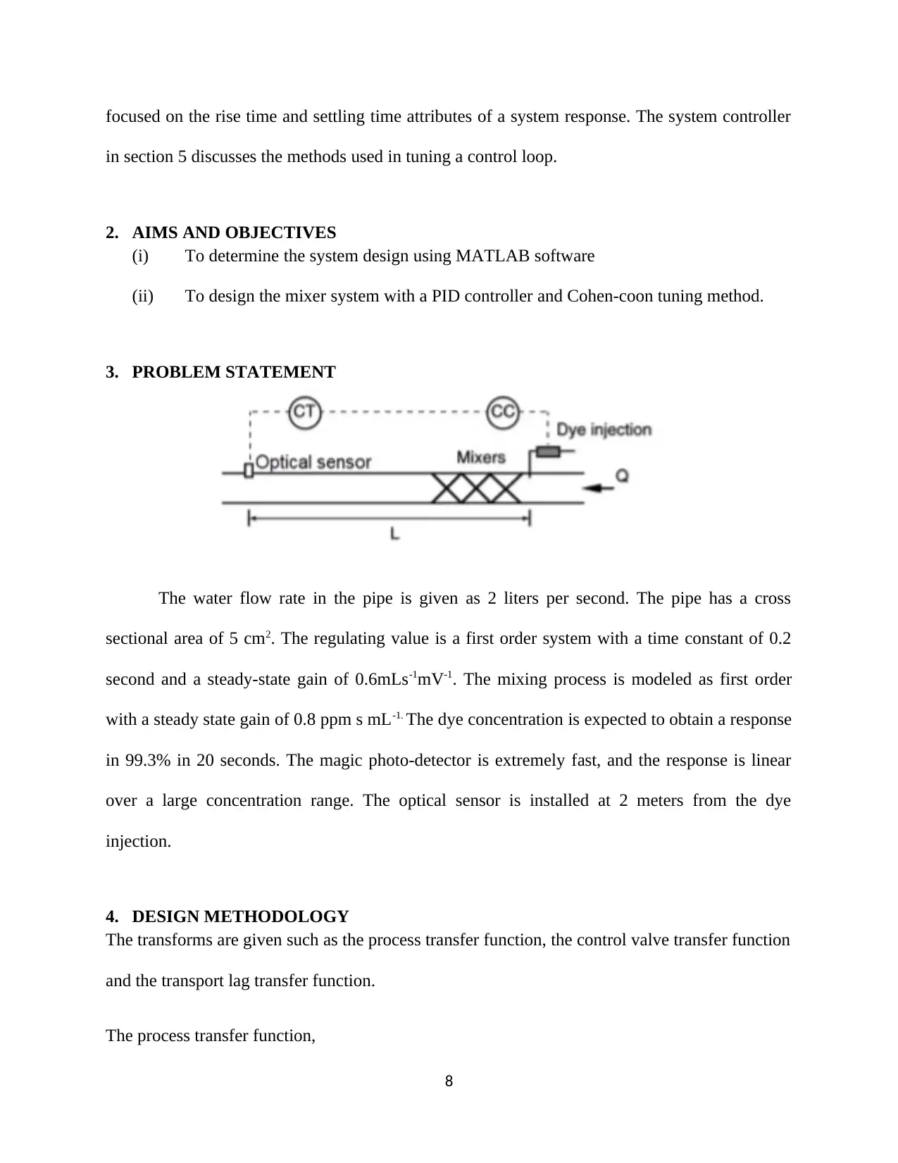
3. PROBLEM STATEMENT
The water flow rate in the pipe is given as 2 liters per second. The pipe has a cross
sectional area of 5 cm2. The regulating value is a first order system with a time constant of 0.2
second and a steady-state gain of 0.6mLs-1mV-1. The mixing process is modeled as first order
with a steady state gain of 0.8 ppm s mL-1. The dye concentration is expected to obtain a response
in 99.3% in 20 seconds. The magic photo-detector is extremely fast, and the response is linear
over a large concentration range. The optical sensor is installed at 2 meters from the dye
injection.
4. DESIGN METHODOLOGY
The transforms are given such as the process transfer function, the control valve transfer function
and the transport lag transfer function.
The process transfer function,
8
in section 5 discusses the methods used in tuning a control loop.
2. AIMS AND OBJECTIVES
(i) To determine the system design using MATLAB software
(ii) To design the mixer system with a PID controller and Cohen-coon tuning method.
3. PROBLEM STATEMENT
The water flow rate in the pipe is given as 2 liters per second. The pipe has a cross
sectional area of 5 cm2. The regulating value is a first order system with a time constant of 0.2
second and a steady-state gain of 0.6mLs-1mV-1. The mixing process is modeled as first order
with a steady state gain of 0.8 ppm s mL-1. The dye concentration is expected to obtain a response
in 99.3% in 20 seconds. The magic photo-detector is extremely fast, and the response is linear
over a large concentration range. The optical sensor is installed at 2 meters from the dye
injection.
4. DESIGN METHODOLOGY
The transforms are given such as the process transfer function, the control valve transfer function
and the transport lag transfer function.
The process transfer function,
8
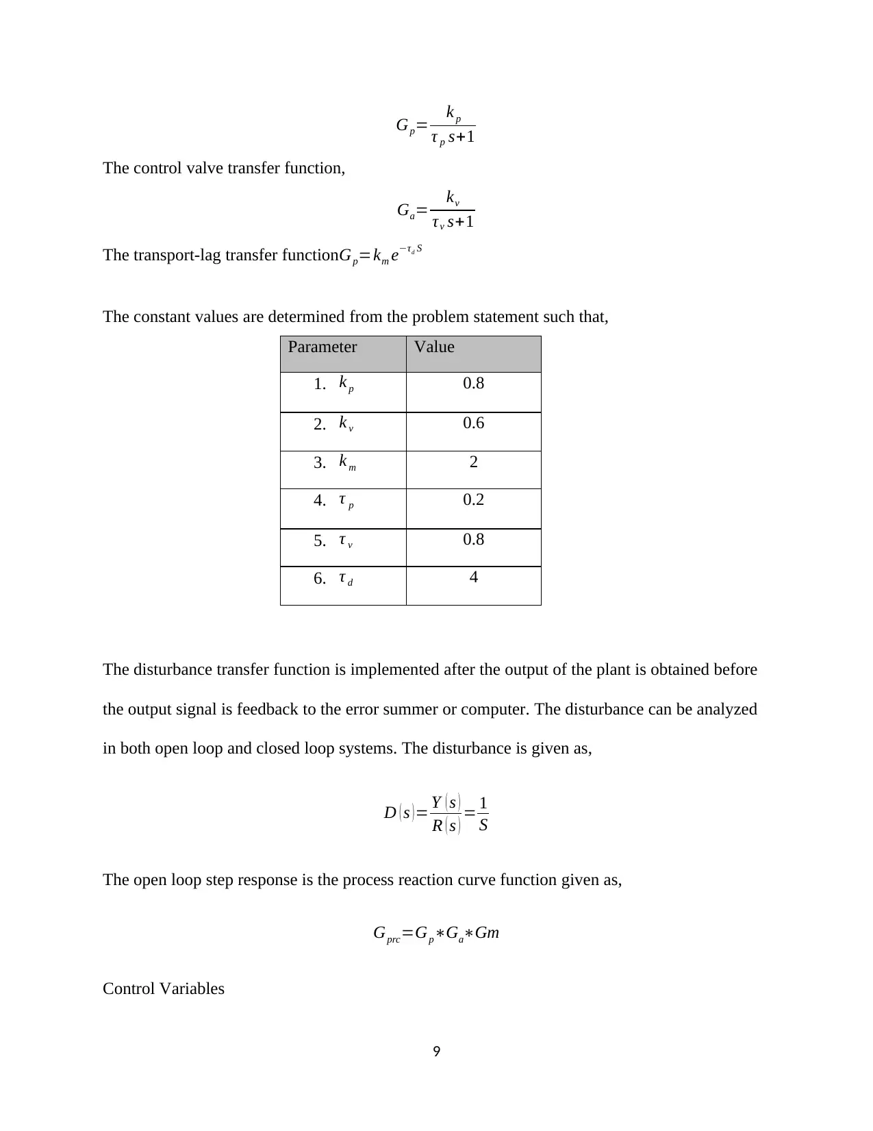
Gp= k p
τ p s+1
The control valve transfer function,
Ga= kv
τv s+1
The transport-lag transfer functionGp=km e−τd S
The constant values are determined from the problem statement such that,
Parameter Value
1. k p 0.8
2. k v 0.6
3. k m 2
4. τ p 0.2
5. τ v 0.8
6. τ d 4
The disturbance transfer function is implemented after the output of the plant is obtained before
the output signal is feedback to the error summer or computer. The disturbance can be analyzed
in both open loop and closed loop systems. The disturbance is given as,
D ( s )= Y ( s )
R ( s ) = 1
S
The open loop step response is the process reaction curve function given as,
Gprc=Gp∗Ga∗Gm
Control Variables
9
⊘ This is a preview!⊘
Do you want full access?
Subscribe today to unlock all pages.
Trusted by 1+ million students worldwide
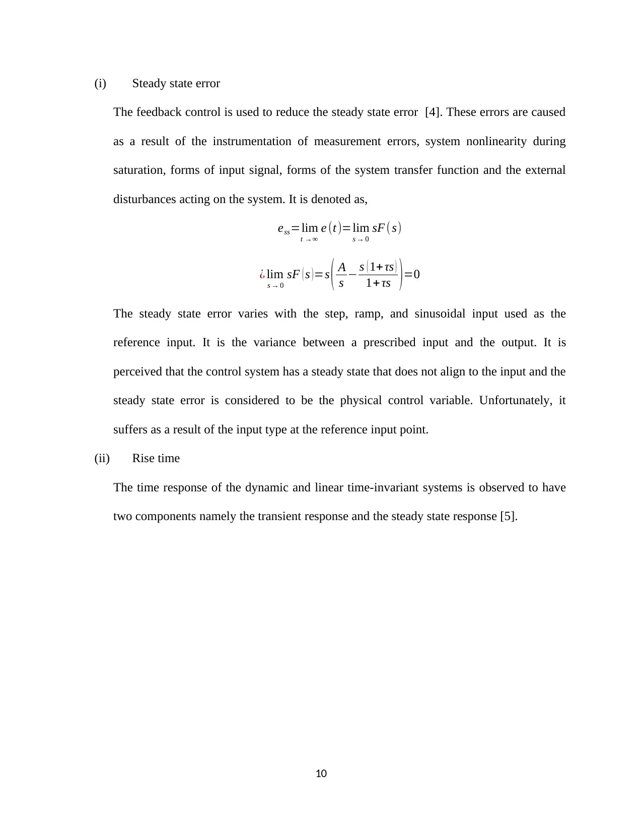
(i) Steady state error
The feedback control is used to reduce the steady state error [4]. These errors are caused
as a result of the instrumentation of measurement errors, system nonlinearity during
saturation, forms of input signal, forms of the system transfer function and the external
disturbances acting on the system. It is denoted as,
ess=lim
t →∞
e (t)=lim
s → 0
sF (s)
¿ lim
s → 0
sF ( s )=s ( A
s − s ( 1+ τs )
1+ τs )=0
The steady state error varies with the step, ramp, and sinusoidal input used as the
reference input. It is the variance between a prescribed input and the output. It is
perceived that the control system has a steady state that does not align to the input and the
steady state error is considered to be the physical control variable. Unfortunately, it
suffers as a result of the input type at the reference input point.
(ii) Rise time
The time response of the dynamic and linear time-invariant systems is observed to have
two components namely the transient response and the steady state response [5].
10
Paraphrase This Document
Need a fresh take? Get an instant paraphrase of this document with our AI Paraphraser
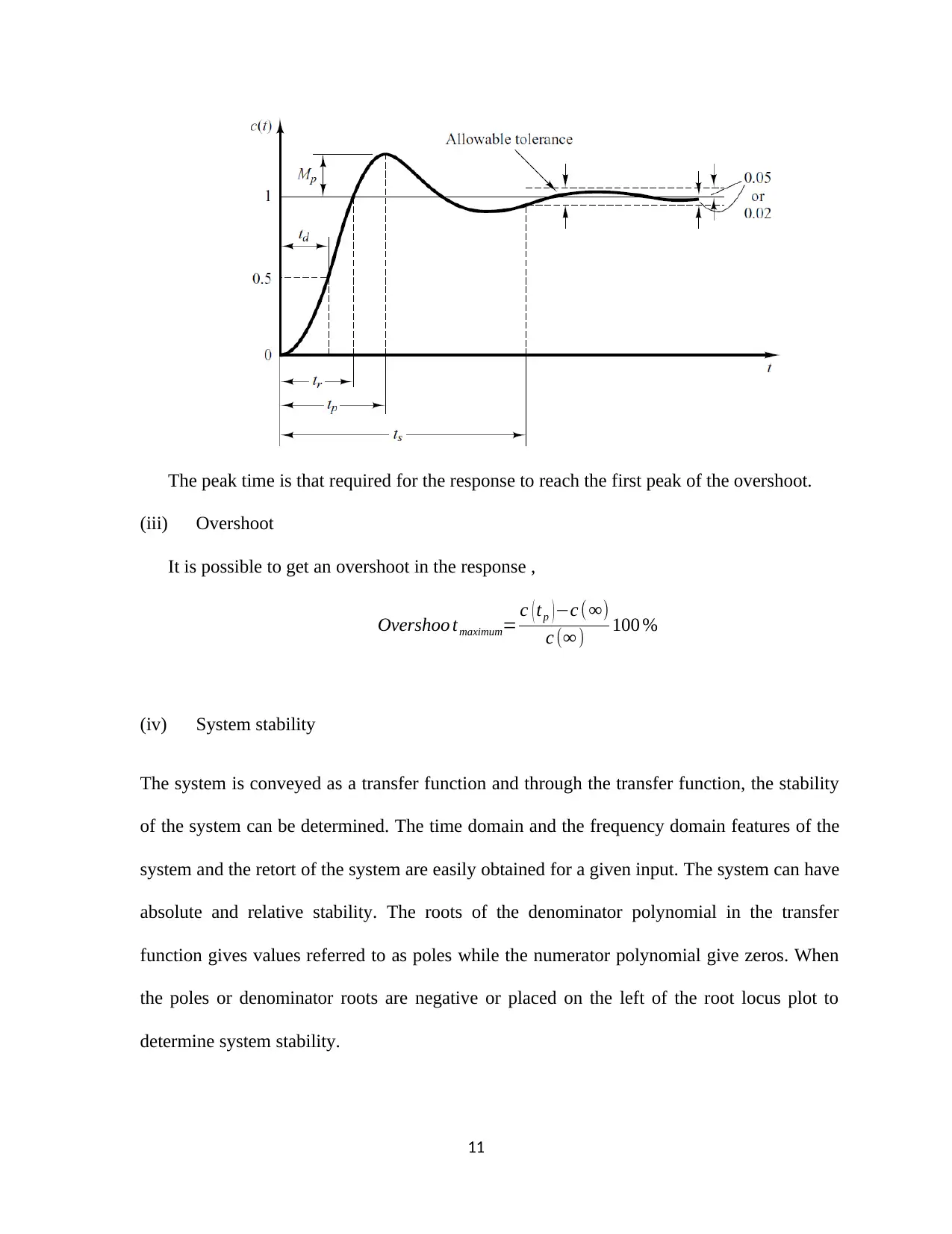
The peak time is that required for the response to reach the first peak of the overshoot.
(iii) Overshoot
It is possible to get an overshoot in the response ,
Overshoo tmaximum= c ( tp ) −c (∞)
c (∞ ) 100 %
(iv) System stability
The system is conveyed as a transfer function and through the transfer function, the stability
of the system can be determined. The time domain and the frequency domain features of the
system and the retort of the system are easily obtained for a given input. The system can have
absolute and relative stability. The roots of the denominator polynomial in the transfer
function gives values referred to as poles while the numerator polynomial give zeros. When
the poles or denominator roots are negative or placed on the left of the root locus plot to
determine system stability.
11
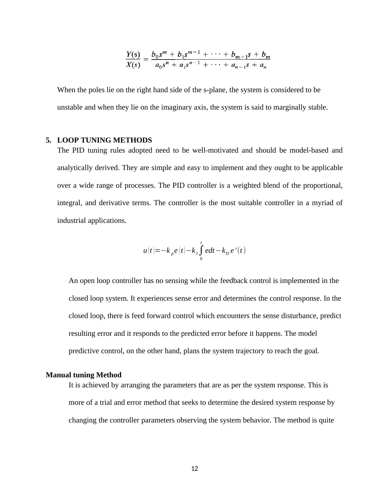
When the poles lie on the right hand side of the s-plane, the system is considered to be
unstable and when they lie on the imaginary axis, the system is said to marginally stable.
5. LOOP TUNING METHODS
The PID tuning rules adopted need to be well-motivated and should be model-based and
analytically derived. They are simple and easy to implement and they ought to be applicable
over a wide range of processes. The PID controller is a weighted blend of the proportional,
integral, and derivative terms. The controller is the most suitable controller in a myriad of
industrial applications.
u ( t ) =−k p e ( t ) −k I∫
0
t
edt −kD e ' (t )
An open loop controller has no sensing while the feedback control is implemented in the
closed loop system. It experiences sense error and determines the control response. In the
closed loop, there is feed forward control which encounters the sense disturbance, predict
resulting error and it responds to the predicted error before it happens. The model
predictive control, on the other hand, plans the system trajectory to reach the goal.
Manual tuning Method
It is achieved by arranging the parameters that are as per the system response. This is
more of a trial and error method that seeks to determine the desired system response by
changing the controller parameters observing the system behavior. The method is quite
12
⊘ This is a preview!⊘
Do you want full access?
Subscribe today to unlock all pages.
Trusted by 1+ million students worldwide
1 out of 28
Related Documents


Your All-in-One AI-Powered Toolkit for Academic Success.
+13062052269
info@desklib.com
Available 24*7 on WhatsApp / Email
![[object Object]](/_next/static/media/star-bottom.7253800d.svg)
Unlock your academic potential
Copyright © 2020–2026 A2Z Services. All Rights Reserved. Developed and managed by ZUCOL.