Statistical Analysis and Regression Report: Manufacturing Industries

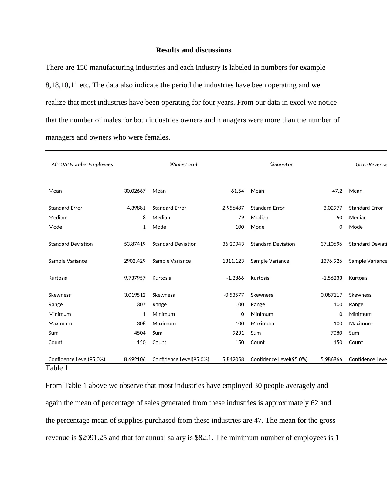
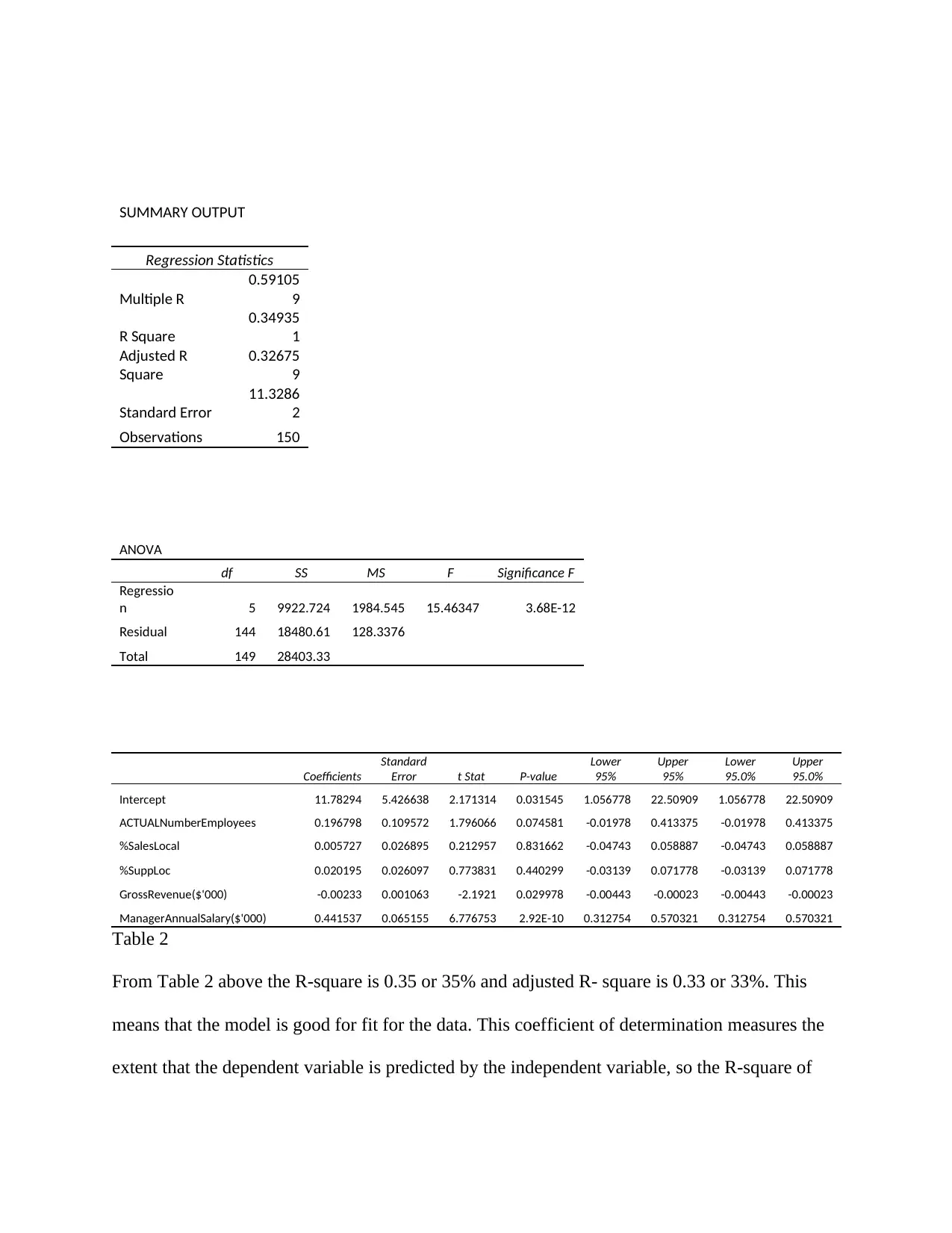
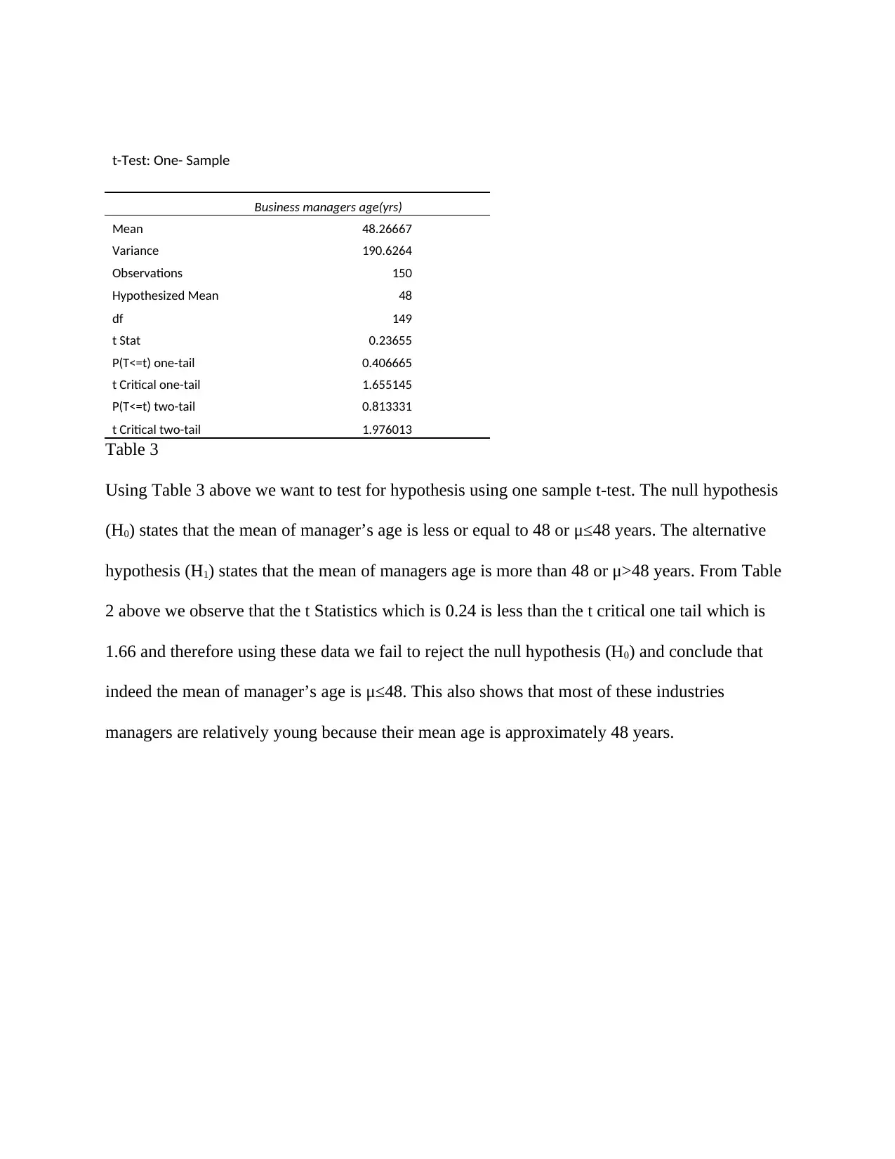
This report presents a statistical analysis of data from 150 manufacturing industries. The analysis includes descriptive statistics such as means, standard deviations, and ranges for variables like the number of employees, sales percentages, gross revenue, manager salaries, and manager ages. Regression analysis is performed to explore the relationships between these variables, revealing an R-squared value of 0.35, indicating the model's ability to explain the variance in manager's age. The report also includes a one-sample t-test to examine the hypothesis that the mean age of managers is less than or equal to 48 years. The findings suggest that the model is significant, with specific coefficients impacting the dependent variable, and the t-test results support the conclusion that the mean age of managers is indeed approximately 48 years or less, indicating a relatively young management demographic across these industries.

Results and discussions
There are 150 manufacturing industries and each industry is labeled in numbers for example
8,18,10,11 etc. The data also indicate the period the industries have been operating and we
realize that most industries have been operating for four years. From our data in excel we notice
that the number of males for both industries owners and managers were more than the number of
managers and owners who were females.
ACTUALNumberEmployees %SalesLocal %SuppLoc GrossRevenue
Mean 30.02667 Mean 61.54 Mean 47.2 Mean
Standard Error 4.39881 Standard Error 2.956487 Standard Error 3.02977 Standard Error
Median 8 Median 79 Median 50 Median
Mode 1 Mode 100 Mode 0 Mode
Standard Deviation 53.87419 Standard Deviation 36.20943 Standard Deviation 37.10696 Standard Deviati
Sample Variance 2902.429 Sample Variance 1311.123 Sample Variance 1376.926 Sample Variance
Kurtosis 9.737957 Kurtosis -1.2866 Kurtosis -1.56233 Kurtosis
Skewness 3.019512 Skewness -0.53577 Skewness 0.087117 Skewness
Range 307 Range 100 Range 100 Range
Minimum 1 Minimum 0 Minimum 0 Minimum
Maximum 308 Maximum 100 Maximum 100 Maximum
Sum 4504 Sum 9231 Sum 7080 Sum
Count 150 Count 150 Count 150 Count
Confidence Level(95.0%) 8.692106 Confidence Level(95.0%) 5.842058 Confidence Level(95.0%) 5.986866 Confidence Leve
Table 1
From Table 1 above we observe that most industries have employed 30 people averagely and
again the mean of percentage of sales generated from these industries is approximately 62 and
the percentage mean of supplies purchased from these industries are 47. The mean for the gross
revenue is $2991.25 and that for annual salary is $82.1. The minimum number of employees is 1

and the maximum is 308. On the managers ages the minimum is 18 years and the maximum is 77
years.

SUMMARY OUTPUT
Regression Statistics
Multiple R
0.59105
9
R Square
0.34935
1
Adjusted R
Square
0.32675
9
Standard Error
11.3286
2
Observations 150
ANOVA
df SS MS F Significance F
Regressio
n 5 9922.724 1984.545 15.46347 3.68E-12
Residual 144 18480.61 128.3376
Total 149 28403.33
Coefficients
Standard
Error t Stat P-value
Lower
95%
Upper
95%
Lower
95.0%
Upper
95.0%
Intercept 11.78294 5.426638 2.171314 0.031545 1.056778 22.50909 1.056778 22.50909
ACTUALNumberEmployees 0.196798 0.109572 1.796066 0.074581 -0.01978 0.413375 -0.01978 0.413375
%SalesLocal 0.005727 0.026895 0.212957 0.831662 -0.04743 0.058887 -0.04743 0.058887
%SuppLoc 0.020195 0.026097 0.773831 0.440299 -0.03139 0.071778 -0.03139 0.071778
GrossRevenue($'000) -0.00233 0.001063 -2.1921 0.029978 -0.00443 -0.00023 -0.00443 -0.00023
ManagerAnnualSalary($'000) 0.441537 0.065155 6.776753 2.92E-10 0.312754 0.570321 0.312754 0.570321
Table 2
From Table 2 above the R-square is 0.35 or 35% and adjusted R- square is 0.33 or 33%. This
means that the model is good for fit for the data. This coefficient of determination measures the
extent that the dependent variable is predicted by the independent variable, so the R-square of

35% means that 35% of the dependent variable (age of managers) is predicted by the
independent variables (number of staff, % saleslocal, %supploc, gross revenue and managers
annual salary). From Table 2 above we can obtain the following multiple model
Y(age of managers)=11.78+0.197*Actualnumber+0.0057*%salesloc+0.02*%supploc-
0.002*gross revenue+0.44*manager annual salary. The significance F is the less than α=0.05
hence the model is significant. The p-value for number of staff, %salesloc, %supploc are greater
than 0.05 hence they are not good for prediction in this model. The coefficients which are
positive are directly proportional to the dependent variable. We only have one coefficient which
is negative and it’s the coefficient of gross revenue, with its shows that a decrease on gross
revenue leads to an increase in manager’s age or they are indirectly proportional. The p-value for
intercept, gross revenue and manager’s annual salary are less than 0.05 hence they can be used
for prediction in this model. The lower and upper value of 95% confidence interval shows that
the coefficient of intercept can take any value within 1.07 to 22.51 and this implies to other
coefficients such as actual number of employs whose lower and upper 95% confidence interval is
-0.02 to0.41, -0.047 to0.059 for % salesloc, -0.03 to0.072 for % supploc, -0.004 to -0.0002 for
gross revenue and 0.31 to 0.57 for managers annual salary.

t-Test: One- Sample
Business managers age(yrs)
Mean 48.26667
Variance 190.6264
Observations 150
Hypothesized Mean 48
df 149
t Stat 0.23655
P(T<=t) one-tail 0.406665
t Critical one-tail 1.655145
P(T<=t) two-tail 0.813331
t Critical two-tail 1.976013
Table 3
Using Table 3 above we want to test for hypothesis using one sample t-test. The null hypothesis
(H0) states that the mean of manager’s age is less or equal to 48 or μ≤48 years. The alternative
hypothesis (H1) states that the mean of managers age is more than 48 or μ>48 years. From Table
2 above we observe that the t Statistics which is 0.24 is less than the t critical one tail which is
1.66 and therefore using these data we fail to reject the null hypothesis (H0) and conclude that
indeed the mean of manager’s age is μ≤48. This also shows that most of these industries
managers are relatively young because their mean age is approximately 48 years.

References
Tradingeconomics.com. (2019). China Non Manufacturing PMI | 2019 | Data | Chart | Calendar |
Forecast. [online] Available at: https://tradingeconomics.com/china/non-manufacturing-pmi [Accessed
21 May 2019].