Solutions for STAT 2006 Assignment 2: Inferential Statistics Problems

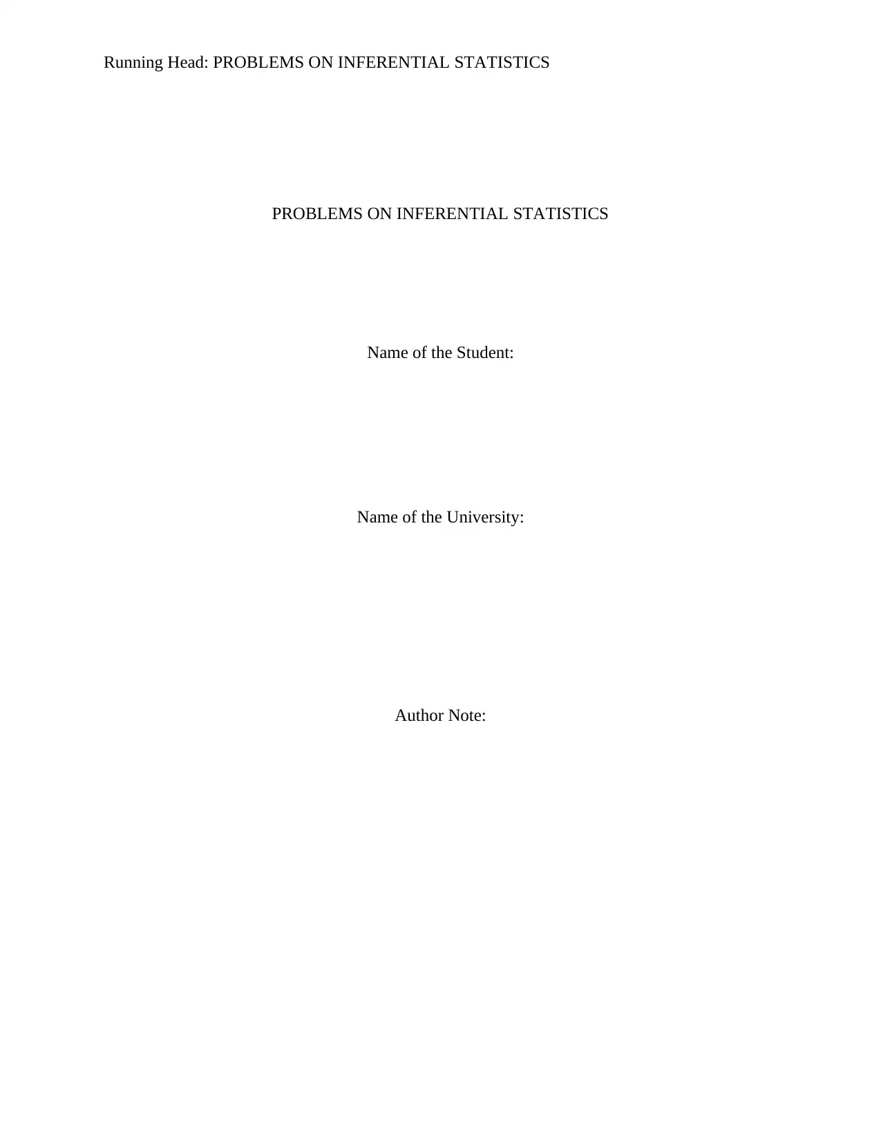
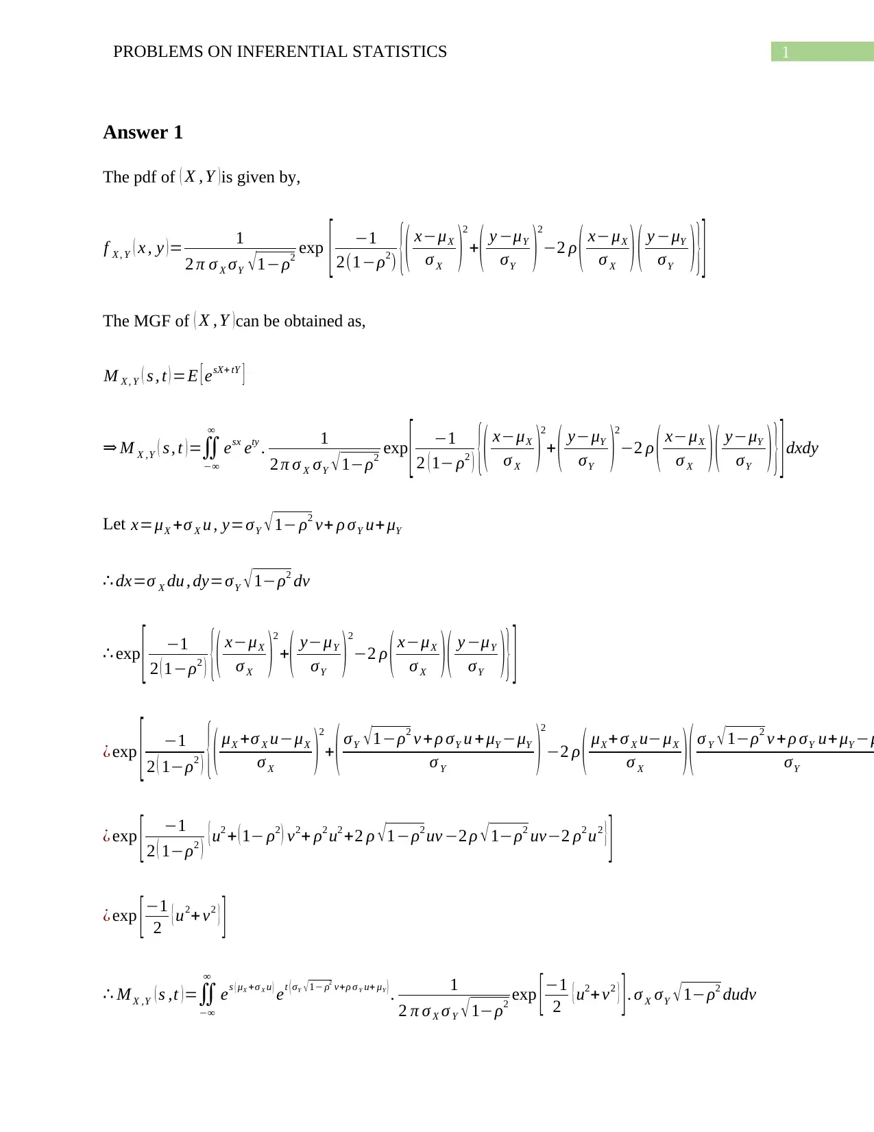
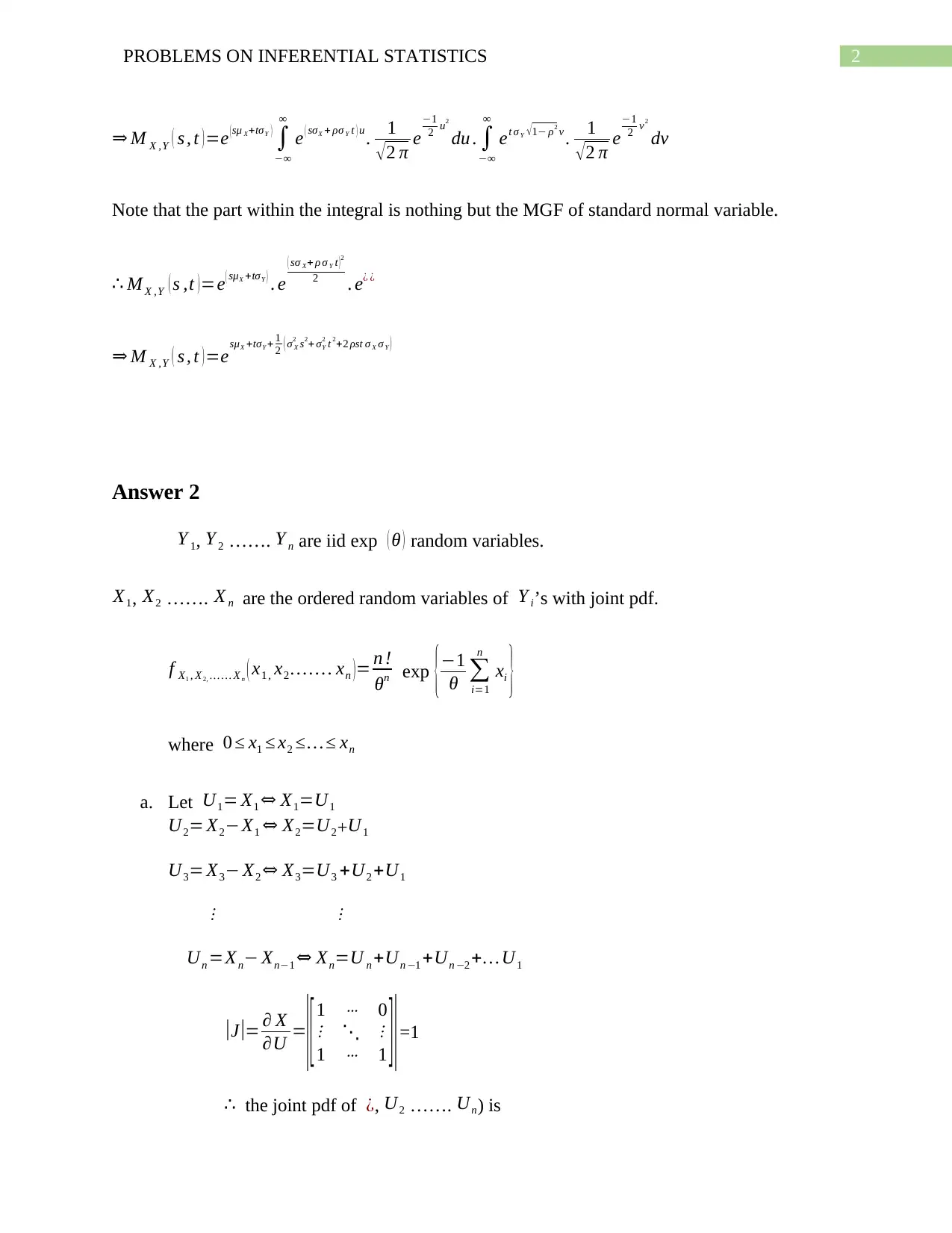
This document presents a comprehensive solution set for an inferential statistics assignment (STAT 2006). It covers a range of problems, including finding the moment-generating function (MGF) for jointly normal random variables, analyzing ordered random variables from an exponential distribution, and determining their independence. The solution also delves into maximum likelihood estimation (MLE), moment estimators, and the application of Chebyshev's inequality. Furthermore, it addresses the properties of bivariate normal distributions, the calculation of sample size, and the analysis of shifted exponential distributions. The document provides detailed step-by-step solutions to each problem, offering valuable insights into the concepts and techniques of inferential statistics. The assignment covers topics such as calculating the MGF, working with exponential distributions, finding joint and marginal probability density functions, and estimating parameters using various methods.

Running Head: PROBLEMS ON INFERENTIAL STATISTICS
PROBLEMS ON INFERENTIAL STATISTICS
Name of the Student:
Name of the University:
Author Note:

1PROBLEMS ON INFERENTIAL STATISTICS
Answer 1
The pdf of ( X , Y )is given by,
f X , Y ( x , y )= 1
2 π σ X σY √1−ρ2 exp [ −1
2(1−ρ2) {( x−μX
σ X )2
+
( y −μY
σY )2
−2 ρ ( x−μX
σ X )( y −μY
σY ) }]
The MGF of ( X , Y )can be obtained as,
M X , Y ( s , t ) =E [ esX+ tY ]
⇒ M X ,Y ( s , t )=∬
−∞
∞
esx ety . 1
2 π σ X σY √1−ρ2 exp [ −1
2 ( 1− ρ2 ) {( x−μX
σ X )2
+ ( y−μY
σY )2
−2 ρ ( x−μX
σ X )( y−μY
σY ) }]dxdy
Let x=μX +σ X u , y=σY √ 1− ρ2 v+ ρ σY u+ μY
∴ dx=σ X du , dy=σY √ 1−ρ2 dv
∴ exp [ −1
2 ( 1−ρ2 ) {( x−μX
σ X )
2
+( y−μY
σY ) 2
−2 ρ ( x−μX
σ X )( y −μY
σY )}]
¿ exp [ −1
2 ( 1−ρ2 ) {( μX +σ X u−μX
σ X )2
+ ( σY √1−ρ2 v + ρ σY u + μY −μY
σ Y )2
−2 ρ ( μX + σ X u−μX
σ X ) ( σ Y √1−ρ2 v + ρ σY u+ μY −μ
σY
¿ exp [ −1
2 ( 1−ρ2 ) { u2 + ( 1− ρ2 ) v2+ ρ2 u2 +2 ρ √ 1−ρ2 uv −2 ρ √ 1−ρ2 uv−2 ρ2 u2 } ]
¿ exp [ −1
2 { u2+ v2 } ]
∴ M X ,Y ( s ,t ) =∬
−∞
∞
es ( μX +σ X u ) et ( σY √ 1− ρ2 v+ρ σ Y u+ μY ) . 1
2 π σ X σ Y √ 1−ρ2 exp [ −1
2 { u2+ v2 } ] . σ X σY √ 1−ρ2 dudv

2PROBLEMS ON INFERENTIAL STATISTICS
⇒ M X ,Y ( s , t ) =e ( sμ X+tσY ) ∫
−∞
∞
e ( sσX + ρσ Y t ) u . 1
√ 2 π e
−1
2 u2
du . ∫
−∞
∞
et σ Y √1− ρ2 v . 1
√ 2 π e
−1
2 v2
dv
Note that the part within the integral is nothing but the MGF of standard normal variable.
∴ M X ,Y ( s ,t ) =e( sμX +tσY ) . e
( sσ X+ ρ σ Y t ) 2
2 . e¿ ¿
⇒ M X ,Y ( s , t ) =esμX +tσY + 1
2 ( σ X
2 s2+ σY
2 t 2+2 ρst σ X σ Y )
Answer 2
Y 1, Y 2 ……. Y n are iid exp ( θ ) random variables.
X1, X2 ……. X n are the ordered random variables of Y i’s with joint pdf.
f X1 , X 2, … … X n ( x1 , x2 … … . xn )= n !
θn exp {−1
θ ∑
i=1
n
xi }
where 0 ≤ x1 ≤ x2 ≤… ≤ xn
a. Let U1= X1 ⇔ X1=U1
U2= X2−X1 ⇔ X2=U2+U1
U3= X3− X2 ⇔ X3=U3 +U2 +U1
⋮ ⋮
Un =Xn− Xn−1 ⇔ Xn=U n +Un −1 +Un −2 +… U1
|J |= ∂ X
∂U =
|[ 1 ⋯ 0
⋮ ⋱ ⋮
1 ⋯ 1 ]|=1
∴ the joint pdf of ¿, U2 ……. Un) is

3PROBLEMS ON INFERENTIAL STATISTICS
g ¿, u2 ……. un) = n !
θn exp −1
θ ¿
= n !
θn exp [−1
θ {n u1+ ( n−1 ) u2 + ( n−2 ) u3+…+un }]
¿ n
θ e
−n
θ u1
. n−1
θ e
−n−1
θ u2
. … … 1
θ e
−1
θ un
b. From the joint pdf, it can be observed that U1, U2 ……. Un are mutually independent.
Marginal distribution of Ui is given by
Ui exp(¿ θ
n−i )¿ i=0 , 1 , 2, ….(n−1)
c. X1 =¿ U1 exp ( θ
n )
E ¿) = θ
n
E ¿) = E[ ∑
i=1
n
Ui ]
= ∑
i=0
n −1 θ
n−ii
¿ θ
n + θ
n−1 +…+θ
¿ θ[1+ 1
2 +…+ 1
n−1 + 1
n ]=Hnθ Hn is the harmonic number
Answer3
Z1 N ( 0,1 ) , Z2 N ( 0,1 ) , Z1 ∧Z2 areindependent .

4PROBLEMS ON INFERENTIAL STATISTICS
X and Y are two random variables defined as,
X =aX Z1+ bX Z2+ cX ∧Y =aY Z1+ bY Z2+ cY
where aX , bX , c X , aY , bY ∧cY are constants.
a. E ( X ) =E ( aX Z1+ bX Z2 + cX )
⇒ E ( X ) =aX E ( Z1 ) +bX E ( Z2 ) +c X
⟹ E ( X ) =aX .0+bX .0+c X [ ∵ E ( Z1 ) =E ( Z2 ) =0 ]
⟹ E ( X ) =cX
E ( Y )=E ( aY Z1+ bY Z2+ cY )
⇒ E ( Y ) =aY E ( Z1 ) +bY E ( Z2 ) +cY
⟹ E ( Y ) =aY .0+bY .0+cY [ ∵ E ( Z1 ) =E ( Z2 ) =0 ]
⟹ E ( Y ) =cY
Var ( X ) =Var ( aX Z1 +bX Z2 +c X )
⇒ Var ( X ) =aX
2 Var ( Z1 ) + bX
2 Var ( Z2 ) [∵ Z1∧Z2 are independent , cov ( Z1 , Z2 ) =0]
⟹ Var ( X )=aX
2 .1+bX
2 .1 [ ∵ Var ( Z1 )=Var ( Z2 ) =1 ]
⟹ Var ( X ) =aX
2 +bX
2
Var ( Y )=Var ( aY Z1 +bY Z2 +cY )
⇒ Var ( Y ) =aY
2 Var ( Z1 ) +bY
2 Var ( Z2 ) [∵ Z1∧Z2 are independent , cov ( Z1 , Z2 ) =0]
⟹ Var ( Y ) =aY
2 .1+bY
2 .1 [ ∵ Var ( Z1 ) =Var ( Z2 ) =1 ]
⟹ Var ( Y ) =aY
2 +bY
2
Now ,Cov ( X ,Y ) =E ( XY ) −E ( X ) E (Y )

5PROBLEMS ON INFERENTIAL STATISTICS
XY = ( aX Z1+ bX Z2 + cX ) . ( aY Z1+ bY Z2+ cY )
⟹ XY =aX aY Z1
2 +bX bY Z2
2+ aX cY Z1+bX cY Z2+ aY cX Z1+bY cX Z2+ aX bY Z1 Z2 +bX aY Z1 Z2+ cX cY
∴ E ( XY )=aX aY E ( Z1
2 )+bX bY E ( Z2
2 )+ aX cY E ( Z1 ) +bX cY E ( Z2 )+ aY c X E ( Z1 ) + bY cX E ( Z2 ) +aX bY E ( Z1 Z2 ) +bX
⟹ E ( XY ) =aX aY .1+ bX bY .1+ aX cY .0+bX cY .0+ aY cX .0+ bY cX .0+ aX bY .0 .0+bX aY .0 .0+c X cY
¿⟹ E ( XY )=aX aY +bX bY +cX cY
∴ Cov ( X , Y )=E ( XY ) −E ( X ) E (Y )
⟹ Cov ( X , Y ) =aX aY +bX bY + cX cY −c X cY
⟹ Cov ( X , Y )=aX aY +bX bY
b. Here it is given that,
aX = √ 1+ ρ
2 σ X , bX = √ 1− ρ
2 σ X , cX =μX ,
aY = √ 1+ρ
2 σY , bY =− √ 1−ρ
2 σY , cY =μY ,
where μX , σ X , μY , σY ∧ρ are constants ,−1 ≤ ρ≤ 1.
∴ E ( X ) =cX =μX , E ( Y ) =cY =μY
Var ( X ) =aX
2 + bX
2 =( √ 1+ ρ
2 σ X )
2
+ ( √ 1−ρ
2 σ X )
2
⟹ Var ( X )= 1+ ρ
2 σ X
2 + 1−ρ
2 σ X
2 =σ X
2
( 1+ ρ
2 + 1−ρ
2 )
⟹ Var ( X )=σ X
2

6PROBLEMS ON INFERENTIAL STATISTICS
Var ( Y ) =aY
2 +bY
2 =( √ 1+ ρ
2 σ Y )
2
+( − √ 1−ρ
2 σY ) 2
⟹ Var ( Y ) =1+ ρ
2 σY
2 + 1−ρ
2 σY
2 =σY
2
( 1+ ρ
2 + 1− ρ
2 )
⟹ Var ( Y ) =σY
2
Cov ( X , Y )=aX aY +bX bY = 1+ ρ
2 σ X σY − 1− ρ
2 σ X σY =ρ σ X σY
Corr ( X ,Y )= Cov (X ,Y )
√Var ( X ) Var (Y )
⟹ Corr ( X , Y )= ρ σ X σY
√σ X
2 σ Y
2
⟹ Corr ( X , Y )= ρ
c. X N ( μX , σ X
2 ) , Y N ( μY , σY
2 ) , corr ( X , Y )= ρ.
Now two independent unit normal variables Z1 , Z2 are generated using the
transformation,
X =σ X Z1+ μ X , Y =σ Y [ ρ Z1 + √1−ρ2 Z2 ]+ μY
∴ Z1= X −μX
σ X
√ 1−ρ2 Z2= Y −μY
σ Y
−ρ Z1 ⇒ Z2= 1
√ 1− ρ2 [ Y −μY
σY
−ρ X −μX
σ X ]
The Jacobian of the transformation,

7PROBLEMS ON INFERENTIAL STATISTICS
J=det [ ∂ ( x , y )
∂ ( z1 , z2 ) ]=det
[ ∂ x
∂ z1
∂ x
∂ z2
∂ y
∂ z1
∂ y
∂ z2
]=det
[ 1
σ X
0
−ρ
σ X √1−ρ2
1
σY √1−ρ2 ]
⇒ J = 1
σ X σY √1−ρ2
Therefore the joint distribution of X and Y is given by,
f ( x , y ) =f ( z1 , z2 )|J|
⇒ f ( x , y ) = 1
2 π exp ¿
⇒ f ( x , y )= 1
2 π σ X σY √1− ρ2 exp [ −1
2 {( x−μX
σ X )2
+ 1
1− ρ2 ( y−μY
σY
−ρ x−μX
σ X )2
}]
⇒ f ( x , y )= 1
2 π σ X σY √1− ρ2 exp [ −1
2(1−ρ2 ) {( x−μX
σ X )2
+ ( y−μY
σ Y )2
−2 ρ ( x−μX
σ X )( y−μY
σY ) }]
Which is the pdf of a bivariate normal distribution.
Hence, the joint distribution of X , Y follows bivariate normal distribution with
parameters μX , μY , σ X , σ Y , ρ .
Answer 4
Xi ' s are iid exp ( θ ) random variables i=1 , 2 ,… . n
Y j ' s are iid exp ( θ ) random variables j=1 ,2 , … . m

8PROBLEMS ON INFERENTIAL STATISTICS
Xi ' s and Y j ' s are independent.
∴ E(X ¿ ¿i)=θ ¿ E(Y ¿ ¿ j)=θ ¿ [ Xi ' s and Y j ' s are independent, covariance is 0]
Var ( X ¿¿ i)=θ2 ¿ Var (Y ¿¿ j)=θ2 ¿
E( X )=E ¿
E(Y )= E ¿
Var ( X )= 1
n2 .∑
i=1
n
var ( X ¿ ¿i)= 1
n2 . n θ2= θ2
n ¿
Var ( Y )= 1
m2 .∑
i=1
m
var (Y ¿ ¿ j)= 1
m2 . mθ2= θ2
m ¿
a. Now, T α =α X + ( 1−α ) Y
E(T α )=αE ( X )+ ( 1−α ) E ¿
¿ αθ + ( 1−α ) θ=θ
V ar ( T α ) =α2 var (X )+(1−α )2 var ¿
¿ α 2 . θ2
n + (1−α )2 . θ2
m
¿ α 2 . θ2
n + (1+α 2−2 α ¿ . θ2
m
¿ θ2 [α 2
( 1
m + 1
n )+ 1
m ( 1−2 α )] ]
b. By Chebyshev’s Inequality,
P [|T α|>ε ] ≤ var ( T α )
ε2 ε > 0

9PROBLEMS ON INFERENTIAL STATISTICS
⇒ P [|T α|>ε ] ≤
θ2
[α2
( 1
m + 1
n )+ 1
m ( 1−2α ) ]
ε2
when m , n→ ∞ , the numerator of the R. H. S. becomes 0.
⇒ P [|T α|>ε ] → 0 as m , n→ ∞
Answer 5
X1, X2 ……. X n are iid U (0,1) random variables
∴ f ( xi ) =1 0< xi ¿ 1
¿ 0 0. w .
a. Let Y =ln X1
⇒ y =ln x1
⇒ x1=e y−∞< y< 0
The Jacobian of thee transformation
|J |=| ∂ x1
∂ y |=ey
∴pdf of y is
f ( y ) =e y−∞< y <0
E ( Y )=∫
−∞
0
y e y dy

10PROBLEMS ON INFERENTIAL STATISTICS
¿ [ y e y−∫1 . ey dy ] −∞
0
¿ [ y e y−e y ]−∞
0
=0−1=−1
E ( Y 2 ) =∫
−∞
0
y2 e y dy
¿ [ y2 e y−2∫ y e y dy ]−∞
0
=[ y2 e y−2 y e y +2 e y ]−∞
0
= 2
var ( Y )=E ¿) - e2 (Y )=2−1=1
b. Xi U ( 0,1 ) ⇒−2 ln Xi χ2
2 ⇒−2∑ ln Xi χ2 n
2
⇒ −2∑ ln Xi−2 n
√ 4 n = 1
√n ∑ ln Xi + √n d
→
N ( 0,1 ) , as n → ∞ , by CLT
lim
n → ∞
P (a ≤ ( X1 X2 X3 … X n )n
−1
2
. en
1
2
≤ b )=¿ lim
n→ ∞
P (lna ≤ 1
√n ∑ ln Xi + √ n≤ lnb )=¿ Φ ( lnb )−Φ ( ln a ) ¿¿
Answer 6
Let X be a random variable with pdf
f ( x ;θ )=θ xθ−1 0 ≤ x ≤ 1, 0<θ <∞

11PROBLEMS ON INFERENTIAL STATISTICS
a. Let ¿, X2 ……. X n ) be an iid random sample of size n drawn from the population with
pdf f ( x ;θ ) ,
If X1, X2 ……. X n takes values x1, x2 , ……. xn , then the likelihood function can be written
as
L ¿ [ x= ( x1 , x2 , … … . xn ) , 0 ≤ xi ≤1,0<θ< ∞ ]
¿ ∏
i=1
n
θ xi
θ−1
¿ θn
∏
i=1
n
xi
θ−1 ----------------------(1)
Taking logarithm (natural logarithm) in both sides of (1)
lnL ( θ∨x )=nlnθ+ ( θ−1 ) ∑
i=1
n
ln xi
The MLE of the parameter θ can be obtained by solving the equation
∂lnL (θ∨x )
∂ θ =0
⇒ ∂
∂ θ [ nlnθ+ ( θ−1 ) ∑
i=1
n
ln xi ] =0
⇒ n
θ +∑
i=1
n
ln xi=0
⇒ n
θ =−∑ ln xi
⇒ θ= −n
∑ ln xi