BUS1BAN Project 2: Inferential Statistics of Mobile Phone Preferences
VerifiedAdded on 2022/11/14
|16
|2852
|2
Project
AI Summary
This project analyzes mobile phone market share and usage among La Trobe University students, utilizing data from a previous research project. It covers inferential statistics, including point estimates and confidence intervals for proportions and means related to gender, iPhone usage, and monthly earnings. The assignment then delves into hypothesis testing to assess the market share of iPhones. Furthermore, it explores the effect of price on preferences between Samsung and Apple phones, employing linear regression to analyze the relationship between price discounts and potential market share. The project includes the interpretation of regression coefficients, the coefficient of determination, and hypothesis testing for the slope of the linear relationship. Finally, the project concludes with a summary of the findings, comparing confidence interval estimates and discussing the underlying statistical concepts and their application to the provided data, including the interpretation of results and conclusions based on the analysis.
Cover Page
Research Project-2: BUS1BAN
Teacher’s Name
Workshop Details
(Time, day, room)
Students ID Number Students Name Student contribution*
(%)
e.g. 50% means the
student will receive 50%
of the marks awarded
Students Signature
*All group members are to exert an equal amount of effort on all questions of the assignment.
Students should not divide sections. If a student has contributed to only some sections, the
contribution of the student should be equal to the marks it carries. A student with less than
100% contribution will receive marks proportional to their contribution.
1
Paraphrase This Document
Need a fresh take? Get an instant paraphrase of this document with our AI Paraphraser
An insight into market share and usage of
mobile phones by students at La Trobe University
Note: Students would continue to be the part of the same group as were
for research project-1 and would be utilising the data from the same
random sample that they have already submitted earlier.
Inferential Statistics
1. Point Estimate and Confidence Interval: (20 marks)
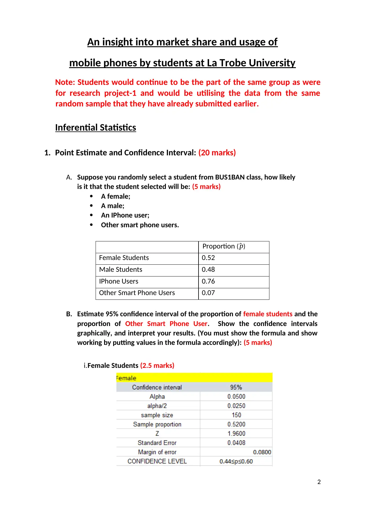
A. Suppose you randomly select a student from BUS1BAN class, how likely
is it that the student selected will be: (5 marks)
A female;
A male;
An IPhone user;
Other smart phone users.
Proportion ( ^p)
Female Students 0.52
Male Students 0.48
IPhone Users 0.76
Other Smart Phone Users 0.07
B. Estimate 95% confidence interval of the proportion of female students and the
proportion of Other Smart Phone User. Show the confidence intervals
graphically, and interpret your results. (You must show the formula and show
working by putting values in the formula accordingly): (5 marks)
i.Female Students (2.5 marks)
2
mobile phones by students at La Trobe University
Note: Students would continue to be the part of the same group as were
for research project-1 and would be utilising the data from the same
random sample that they have already submitted earlier.
Inferential Statistics
1. Point Estimate and Confidence Interval: (20 marks)
A. Suppose you randomly select a student from BUS1BAN class, how likely
is it that the student selected will be: (5 marks)
A female;
A male;
An IPhone user;
Other smart phone users.
Proportion ( ^p)
Female Students 0.52
Male Students 0.48
IPhone Users 0.76
Other Smart Phone Users 0.07
B. Estimate 95% confidence interval of the proportion of female students and the
proportion of Other Smart Phone User. Show the confidence intervals
graphically, and interpret your results. (You must show the formula and show
working by putting values in the formula accordingly): (5 marks)
i.Female Students (2.5 marks)
2
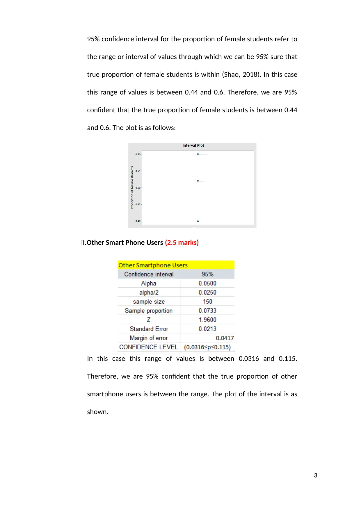
95% confidence interval for the proportion of female students refer to
the range or interval of values through which we can be 95% sure that
true proportion of female students is within (Shao, 2018). In this case
this range of values is between 0.44 and 0.6. Therefore, we are 95%
confident that the true proportion of female students is between 0.44
and 0.6. The plot is as follows:
ii.Other Smart Phone Users (2.5 marks)
In this case this range of values is between 0.0316 and 0.115.
Therefore, we are 95% confident that the true proportion of other
smartphone users is between the range. The plot of the interval is as
shown.
3
⊘ This is a preview!⊘
Do you want full access?
Subscribe today to unlock all pages.
Trusted by 1+ million students worldwide
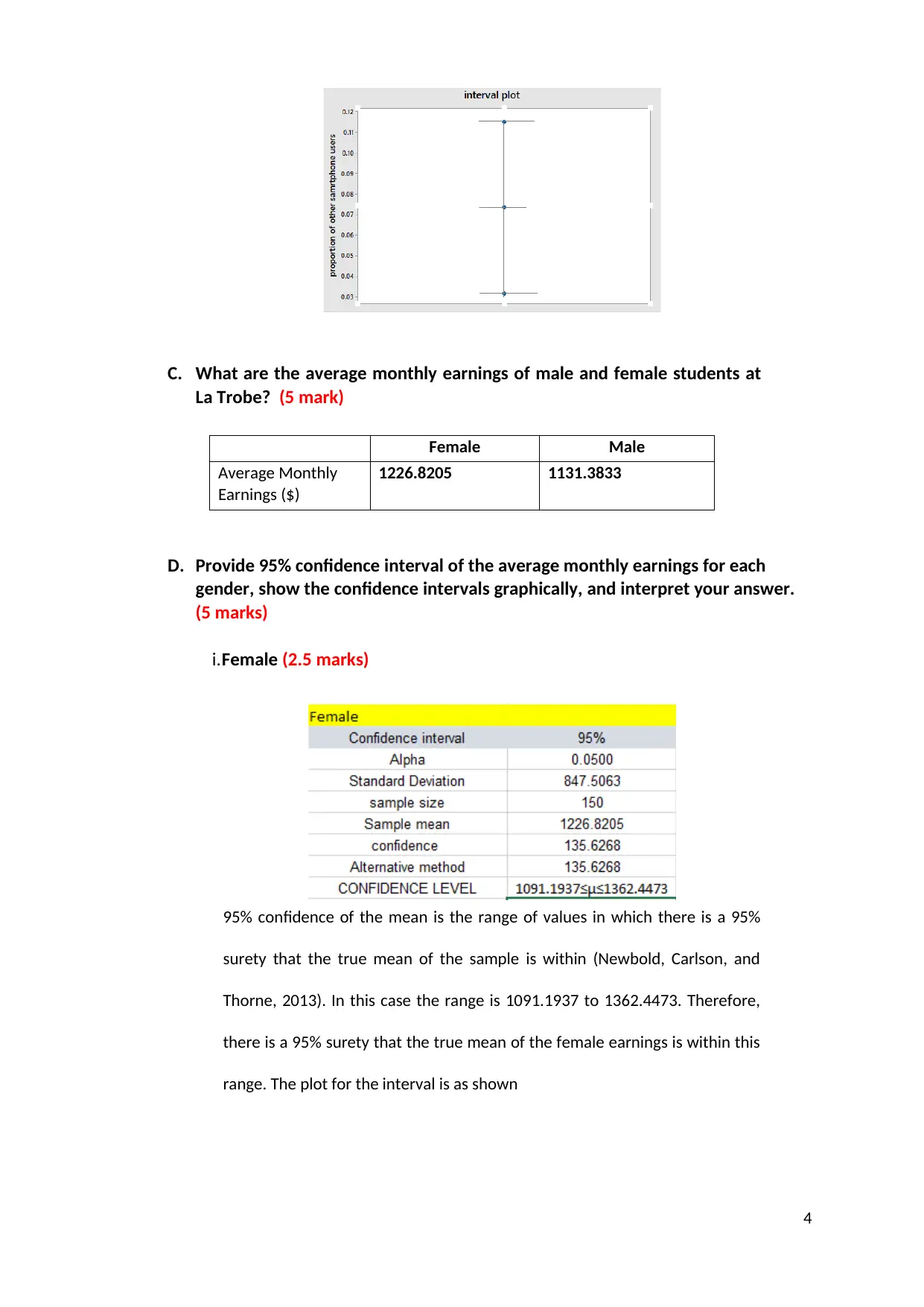
C. What are the average monthly earnings of male and female students at
La Trobe? (5 mark)
Female Male
Average Monthly
Earnings ($)
1226.8205 1131.3833
D. Provide 95% confidence interval of the average monthly earnings for each
gender, show the confidence intervals graphically, and interpret your answer.
(5 marks)
i.Female (2.5 marks)
95% confidence of the mean is the range of values in which there is a 95%
surety that the true mean of the sample is within (Newbold, Carlson, and
Thorne, 2013). In this case the range is 1091.1937 to 1362.4473. Therefore,
there is a 95% surety that the true mean of the female earnings is within this
range. The plot for the interval is as shown
4
Paraphrase This Document
Need a fresh take? Get an instant paraphrase of this document with our AI Paraphraser
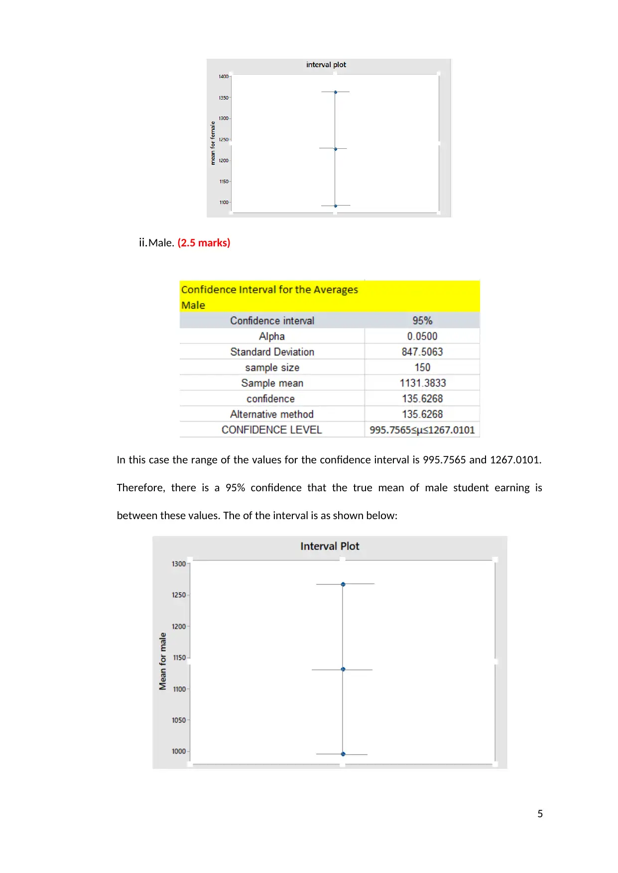
ii.Male. (2.5 marks)
In this case the range of the values for the confidence interval is 995.7565 and 1267.0101.
Therefore, there is a 95% confidence that the true mean of male student earning is
between these values. The of the interval is as shown below:
5
In this case the range of the values for the confidence interval is 995.7565 and 1267.0101.
Therefore, there is a 95% confidence that the true mean of male student earning is
between these values. The of the interval is as shown below:
5
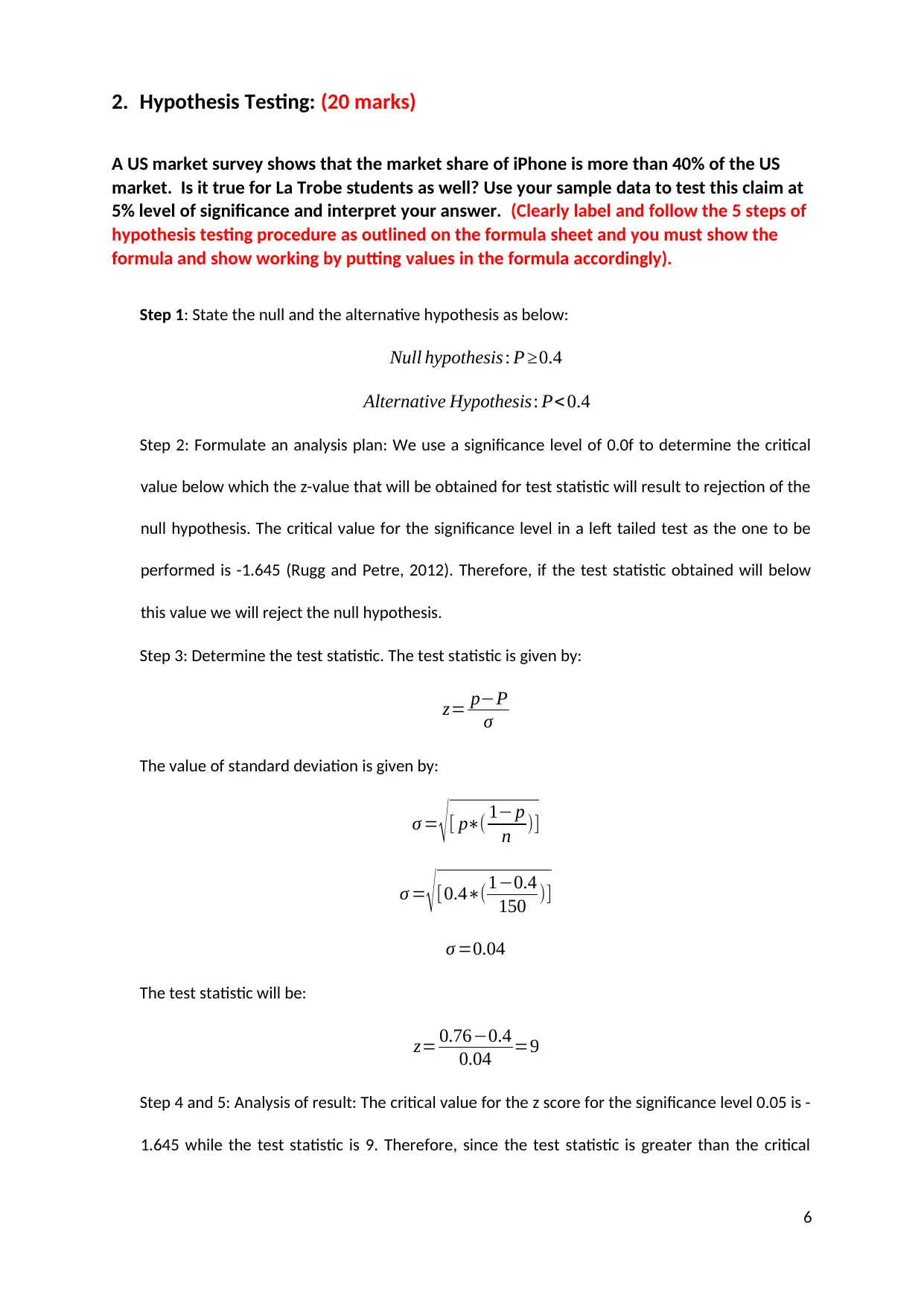
2. Hypothesis Testing: (20 marks)
A US market survey shows that the market share of iPhone is more than 40% of the US
market. Is it true for La Trobe students as well? Use your sample data to test this claim at
5% level of significance and interpret your answer. (Clearly label and follow the 5 steps of
hypothesis testing procedure as outlined on the formula sheet and you must show the
formula and show working by putting values in the formula accordingly).
Step 1: State the null and the alternative hypothesis as below:
Null hypothesis : P ≥0.4
Alternative Hypothesis: P< 0.4
Step 2: Formulate an analysis plan: We use a significance level of 0.0f to determine the critical
value below which the z-value that will be obtained for test statistic will result to rejection of the
null hypothesis. The critical value for the significance level in a left tailed test as the one to be
performed is -1.645 (Rugg and Petre, 2012). Therefore, if the test statistic obtained will below
this value we will reject the null hypothesis.
Step 3: Determine the test statistic. The test statistic is given by:
z= p−P
σ
The value of standard deviation is given by:
σ = √[ p∗( 1− p
n )]
σ = √[0.4∗(1−0.4
150 )]
σ =0.04
The test statistic will be:
z= 0.76−0.4
0.04 =9
Step 4 and 5: Analysis of result: The critical value for the z score for the significance level 0.05 is -
1.645 while the test statistic is 9. Therefore, since the test statistic is greater than the critical
6
⊘ This is a preview!⊘
Do you want full access?
Subscribe today to unlock all pages.
Trusted by 1+ million students worldwide
value or is towards the right of the critical value, we do not reject the null hypothesis and can
confidently conclude that market share of iPhone is more than 40% for the students.
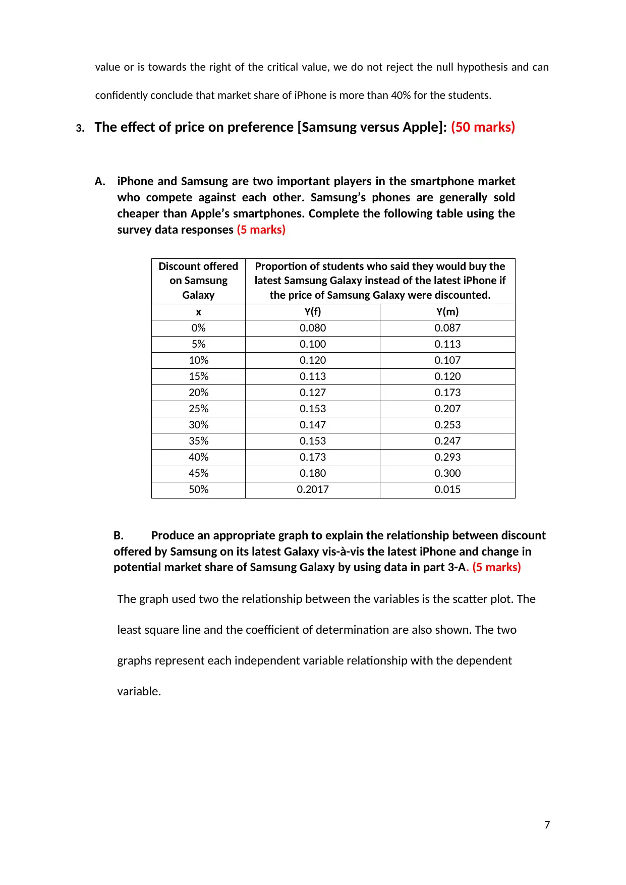
3. The effect of price on preference [Samsung versus Apple]: (50 marks)
A. iPhone and Samsung are two important players in the smartphone market
who compete against each other. Samsung’s phones are generally sold
cheaper than Apple’s smartphones. Complete the following table using the
survey data responses (5 marks)
Discount offered
on Samsung
Galaxy
Proportion of students who said they would buy the
latest Samsung Galaxy instead of the latest iPhone if
the price of Samsung Galaxy were discounted.
x Y(f) Y(m)
0% 0.080 0.087
5% 0.100 0.113
10% 0.120 0.107
15% 0.113 0.120
20% 0.127 0.173
25% 0.153 0.207
30% 0.147 0.253
35% 0.153 0.247
40% 0.173 0.293
45% 0.180 0.300
50% 0.2017 0.015
B. Produce an appropriate graph to explain the relationship between discount
offered by Samsung on its latest Galaxy vis-à-vis the latest iPhone and change in
potential market share of Samsung Galaxy by using data in part 3-A. (5 marks)
The graph used two the relationship between the variables is the scatter plot. The
least square line and the coefficient of determination are also shown. The two
graphs represent each independent variable relationship with the dependent
variable.
7
confidently conclude that market share of iPhone is more than 40% for the students.
3. The effect of price on preference [Samsung versus Apple]: (50 marks)
A. iPhone and Samsung are two important players in the smartphone market
who compete against each other. Samsung’s phones are generally sold
cheaper than Apple’s smartphones. Complete the following table using the
survey data responses (5 marks)
Discount offered
on Samsung
Galaxy
Proportion of students who said they would buy the
latest Samsung Galaxy instead of the latest iPhone if
the price of Samsung Galaxy were discounted.
x Y(f) Y(m)
0% 0.080 0.087
5% 0.100 0.113
10% 0.120 0.107
15% 0.113 0.120
20% 0.127 0.173
25% 0.153 0.207
30% 0.147 0.253
35% 0.153 0.247
40% 0.173 0.293
45% 0.180 0.300
50% 0.2017 0.015
B. Produce an appropriate graph to explain the relationship between discount
offered by Samsung on its latest Galaxy vis-à-vis the latest iPhone and change in
potential market share of Samsung Galaxy by using data in part 3-A. (5 marks)
The graph used two the relationship between the variables is the scatter plot. The
least square line and the coefficient of determination are also shown. The two
graphs represent each independent variable relationship with the dependent
variable.
7
Paraphrase This Document
Need a fresh take? Get an instant paraphrase of this document with our AI Paraphraser
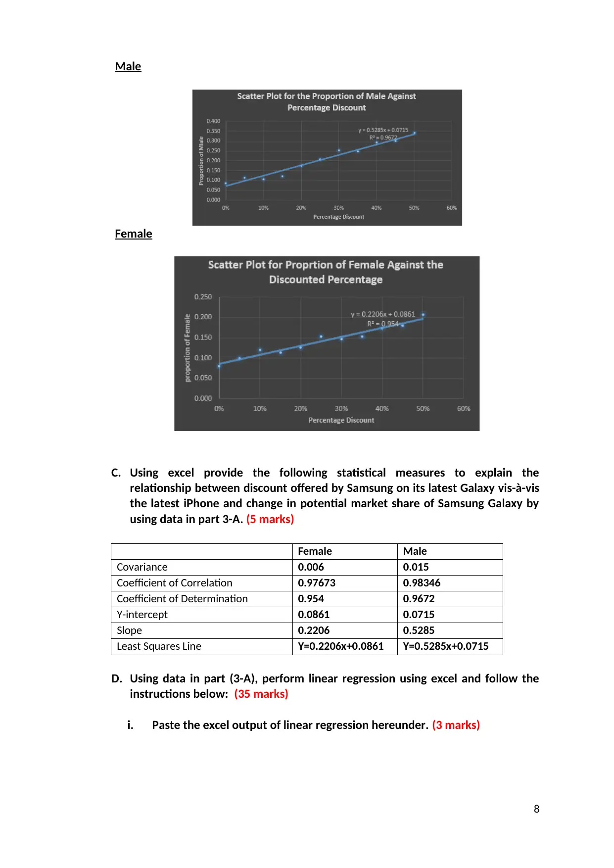
Male
Female
C. Using excel provide the following statistical measures to explain the
relationship between discount offered by Samsung on its latest Galaxy vis-à-vis
the latest iPhone and change in potential market share of Samsung Galaxy by
using data in part 3-A. (5 marks)
Female Male
Covariance 0.006 0.015
Coefficient of Correlation 0.97673 0.98346
Coefficient of Determination 0.954 0.9672
Y-intercept 0.0861 0.0715
Slope 0.2206 0.5285
Least Squares Line Y=0.2206x+0.0861 Y=0.5285x+0.0715
D. Using data in part (3-A), perform linear regression using excel and follow the
instructions below: (35 marks)
i. Paste the excel output of linear regression hereunder. (3 marks)
8
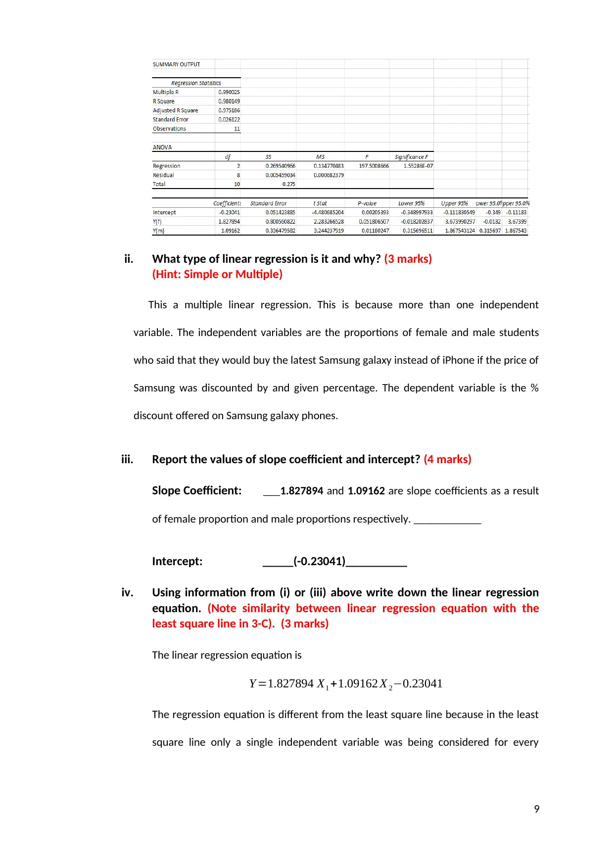
ii. What type of linear regression is it and why? (3 marks)
(Hint: Simple or Multiple)
This a multiple linear regression. This is because more than one independent
variable. The independent variables are the proportions of female and male students
who said that they would buy the latest Samsung galaxy instead of iPhone if the price of
Samsung was discounted by and given percentage. The dependent variable is the %
discount offered on Samsung galaxy phones.
iii. Report the values of slope coefficient and intercept? (4 marks)
Slope Coefficient: ___1.827894 and 1.09162 are slope coefficients as a result
of female proportion and male proportions respectively. ____________
Intercept: _____(-0.23041)__________
iv. Using information from (i) or (iii) above write down the linear regression
equation. (Note similarity between linear regression equation with the
least square line in 3-C). (3 marks)
The linear regression equation is
Y =1.827894 X1 +1.09162 X 2−0.23041
The regression equation is different from the least square line because in the least
square line only a single independent variable was being considered for every
9
⊘ This is a preview!⊘
Do you want full access?
Subscribe today to unlock all pages.
Trusted by 1+ million students worldwide
instance unlike in the multiple linear regression equation where the two
independent variables are considered simultaneously.
v. Interpret Intercept: (3 marks)
The intercept is -0.23041. It indicates the value of the dependent variable if
the value of both the independent variables would be zero. For example, in
this case, the regression equation is:
Y =1.827894 X1 +1.09162 X 2−0.23041
If the two independent variables would be zero, then
Y =1.827894∗0+1.09162∗0−0.23041
Y =−0.23041
vi. Interpret Slope Coefficient: (3 marks)
The slopes are coefficients of the independent variable. The first
independent variable is the proportion of female students while the second
independent variable is the proportion of male students; both of which
would prefer buying Samsung galaxy for a given percentage discount. The
coefficients and hence the slopes are 1.828 and 1.092 respectively. They
both indicate the magnitude with which the independent variables influence
the dependent variable. For example, if the first independent variable was 1
and the second independent variable was 2. Then the value of the
dependent variable would be:
Y =1.827894∗1+1.09162∗2−0.23041
Y =3.7807
vii. Interpret Coefficient of determination: (3 marks)
10
Paraphrase This Document
Need a fresh take? Get an instant paraphrase of this document with our AI Paraphraser
The coefficient of determination is the R-squared value and is 0.9801. Its
purpose is to measure the explained variation. In this case the value 0.9801
indicates that 98.01% of the given variation in the proportions of the
students can be explained by the percentage discount in the price of
Samsung galaxy. In simples, 0.9801 coefficient of determination means that
98.01 of the predictions are explained by the regression model.
viii. What is the relationship between Coefficient of Correlation and Coefficient
of Determination? Compute Coefficient of Correlation by using Coefficient
of Determination (Show working): (3 marks)
Coefficient of correction is used to determine the presence and the strength
of a linear relationship whereas the coefficient of determination is used to
determine the explained variation by the model. The coefficient of
determination= 0.9801 indicates that 98.01% of the predictions are
explained by the model (Tuffery, 2013). The value of the coefficient of
correlation of the square root of the coefficient of determination as follows:
R= √ R2
R= √0.9801
R=0.99
The coefficient of correlation shows that there is a strong positive linear
relationship between the independent and the dependent variables.
ix. Perform hypothesis testing to test slope for linear relationship by using t-
statistics in the excel output. (Clearly label and follow the 5 steps of
hypothesis testing procedure as outlined on the formula sheet and you
11
must show the formula and show working by putting values in the formula
accordingly). (10 marks)
Step 1: We state the null hypothesis and the alternative hypothesis as
follows;
null hypothesis Ho : Bo=0
Alternative hypothesis : Hi :Bi ≠ 0
Step 2: We formulate and analysis plan: A default significance level of 0.05%
is chosen and we can apply the t-test to examine whether the slope for the
linear relationship is significantly different from zero (Rumsey, 2015).
Step 3: We analyse the sample data: This is done to determine the slope, the
standard error, the t-test statistic and the degrees of freedom. The table
below summarizes the result:
Slope DF SE T-STAT
1.827894 10 0.80056 2.283267
1.09162 10 0.33648 3.24423
Step 4: Determine the p-values: it is the probability that the test statistic
having 10 degrees of freedom will be greater than 2.28 and 3.24 respectively
on the positive and the negative side since it’s a two tailed test. The p values
from the t-distribution table are 0.05 and 0.01 respectively.
Step 5: Interpretation of results: Since the first p-value is slightly greater than
the significance level of 0.05 if not rounded off, then we do not reject the
null hypothesis and can conclude that the slope is zero. Since the second
slope (0.01) is less than significance level we reject the null hypothesis and
conclude that the mean is different from zero.
12
⊘ This is a preview!⊘
Do you want full access?
Subscribe today to unlock all pages.
Trusted by 1+ million students worldwide
1 out of 16
Related Documents


Your All-in-One AI-Powered Toolkit for Academic Success.
+13062052269
info@desklib.com
Available 24*7 on WhatsApp / Email
![[object Object]](/_next/static/media/star-bottom.7253800d.svg)
Unlock your academic potential
Copyright © 2020–2026 A2Z Services. All Rights Reserved. Developed and managed by ZUCOL.