UCD STAT20100: Inferential Statistics Assignment 2, Semester 2, 2020

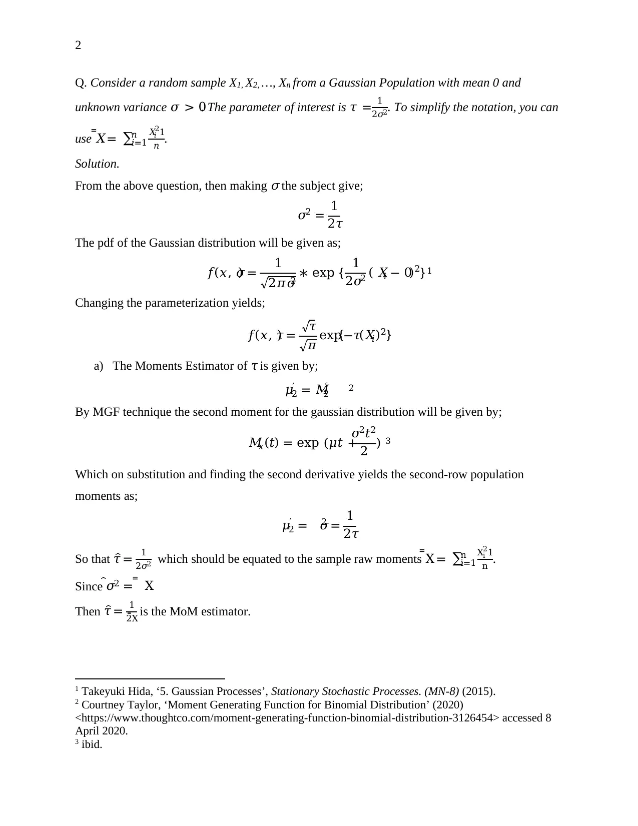
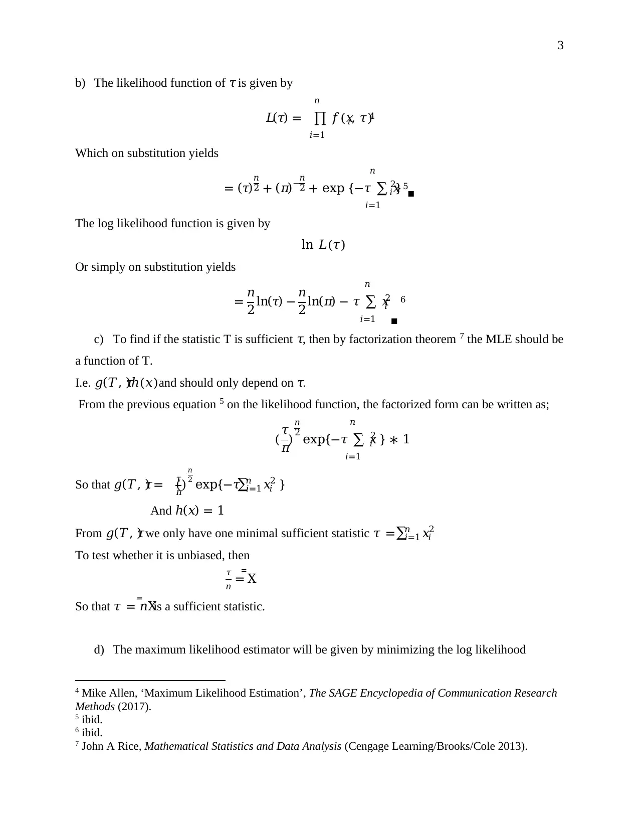
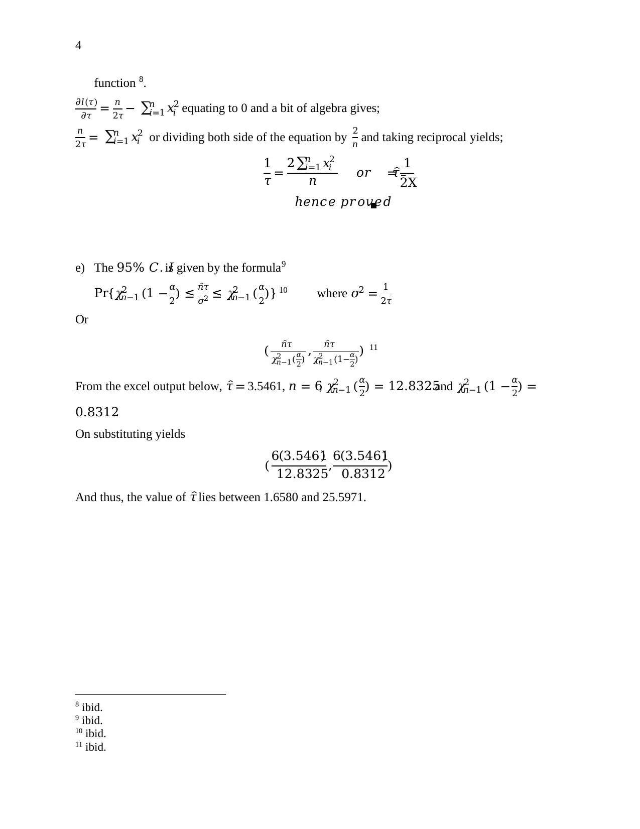
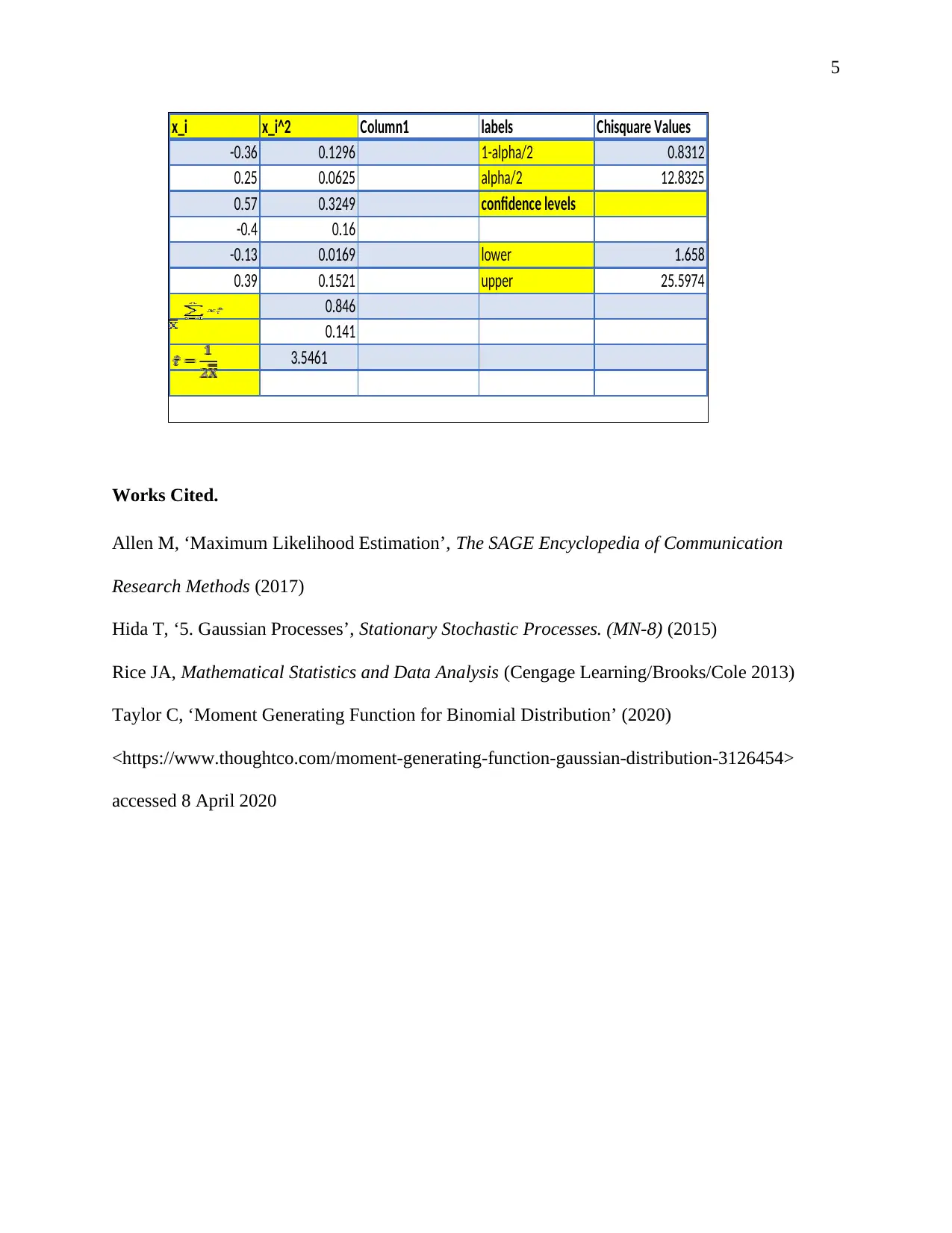
This document presents a complete solution to an Inferential Statistics assignment, focusing on a random sample from a Gaussian population. The solution begins by determining the method of moments estimator for the parameter τ, utilizing the second non-central moment. It then derives the likelihood and log-likelihood functions for τ. The assignment proceeds to demonstrate that nX is a sufficient statistic for τ, followed by a proof that the maximum likelihood estimator for τ is τ̂ = 1/(2X). Finally, the solution calculates a 95% confidence interval based on a given sample realization, providing the necessary calculations and Excel output to support the results. The assignment comprehensively addresses key concepts in inferential statistics, including estimation, likelihood, sufficiency, and confidence intervals.

1
INFERENTIAL STATISTICS
Name of the Student
Name of the University
Author’s Note.

2
Q. Consider a random sample X1, X2, …, Xn from a Gaussian Population with mean 0 and
unknown variance 𝜎 > 0. The parameter of interest is 𝜏 = 1
2𝜎2. To simplify the notation, you can
use 𝑋̿= ∑ 𝑋𝑖
21
𝑛
𝑛
𝑖=1 .
Solution.
From the above question, then making 𝜎 the subject give;
𝜎2 = 1
2𝜏
The pdf of the Gaussian distribution will be given as;
𝑓(𝑥, 𝜎) = 1
√2𝜋𝜎2 ∗ exp {−1
2𝜎2 ( 𝑋𝑖 − 0)2} 1
Changing the parameterization yields;
𝑓(𝑥, 𝜏) = √𝜏
√𝜋 exp{−𝜏(𝑋𝑖)2}
a) The Moments Estimator of 𝜏 is given by;
𝜇2
′ = 𝑀2
′ 2
By MGF technique the second moment for the gaussian distribution will be given by;
𝑀𝑥(𝑡) = exp (𝜇𝑡 +
𝜎2𝑡2
2 ) 3
Which on substitution and finding the second derivative yields the second-row population
moments as;
𝜇2
′ = 𝜎2 = 1
2𝜏
So that 𝜏̂= 1
2𝜎2 which should be equated to the sample raw moments X̿ = ∑ Xi
21
n
n
i=1 .
Since 𝜎2̂ = X̿
Then 𝜏̂= 1
2X̿ is the MoM estimator.
1 Takeyuki Hida, ‘5. Gaussian Processes’, Stationary Stochastic Processes. (MN-8) (2015).
2 Courtney Taylor, ‘Moment Generating Function for Binomial Distribution’ (2020)
<https://www.thoughtco.com/moment-generating-function-binomial-distribution-3126454> accessed 8
April 2020.
3 ibid.

3
b) The likelihood function of 𝜏 is given by
𝐿(𝜏) = ∏ 𝑓(𝑥𝑖, 𝜏)
𝑛
𝑖=1
4
Which on substitution yields
= (𝜏)𝑛
2 + (𝜋)−𝑛
2 + exp {−𝜏 ∑ 𝑥𝑖
2
𝑛
𝑖=1
} 5∎
The log likelihood function is given by
ln 𝐿(𝜏)
Or simply on substitution yields
= 𝑛
2 ln(𝜏) − 𝑛
2 ln(𝜋) − 𝜏 ∑ 𝑥𝑖
2
𝑛
𝑖=1 ∎
6
c) To find if the statistic T is sufficient 𝜏, then by factorization theorem 7 the MLE should be
a function of T.
I.e. 𝑔(𝑇, 𝜏)ℎ(𝑥)and should only depend on 𝜏.
From the previous equation 5 on the likelihood function, the factorized form can be written as;
( 𝜏
𝜋
)
𝑛
2 exp{−𝜏 ∑ 𝑥𝑖
2
𝑛
𝑖=1
} ∗ 1
So that 𝑔(𝑇, 𝜏) = (
𝜏
𝜋)
𝑛
2 exp{−𝜏∑ 𝑥𝑖
2𝑛
𝑖=1 }
And ℎ(𝑥) = 1
From 𝑔(𝑇, 𝜏) we only have one minimal sufficient statistic 𝜏 =∑ 𝑥𝑖
2𝑛
𝑖=1
To test whether it is unbiased, then
𝜏
𝑛 = X̿
So that 𝜏 = 𝑛X̿is a sufficient statistic.
d) The maximum likelihood estimator will be given by minimizing the log likelihood
4 Mike Allen, ‘Maximum Likelihood Estimation’, The SAGE Encyclopedia of Communication Research
Methods (2017).
5 ibid.
6 ibid.
7 John A Rice, Mathematical Statistics and Data Analysis (Cengage Learning/Brooks/Cole 2013).

4
function 8.
𝜕𝑙(𝜏)
𝜕𝜏 = 𝑛
2𝜏 − ∑ 𝑥𝑖
2𝑛
𝑖=1 equating to 0 and a bit of algebra gives;
𝑛
2𝜏 = ∑ 𝑥𝑖
2𝑛
𝑖=1 or dividing both side of the equation by 2
𝑛 and taking reciprocal yields;
1
𝜏 = 2∑ 𝑥𝑖
2𝑛
𝑖=1
𝑛 𝑜𝑟 𝜏̂= 1
2X̿
ℎ𝑒𝑛𝑐𝑒 𝑝𝑟𝑜𝑣𝑒𝑑∎
e) The 95% 𝐶. 𝐼is given by the formula9
Pr{𝜒𝑛−1
2 (1 −𝛼
2) ≤ 𝑛𝜏̂
𝜎2 ≤ 𝜒𝑛−1
2 (𝛼
2)} 10 where 𝜎2 = 1
2𝜏
Or
( 𝑛𝜏̂
𝜒𝑛−1
2 (𝛼
2) , 𝑛𝜏̂
𝜒𝑛−1
2 (1−𝛼
2)) 11
From the excel output below, 𝜏̂= 3.5461, 𝑛 = 6, 𝜒𝑛−1
2 (𝛼
2) = 12.8325and 𝜒𝑛−1
2 (1 −𝛼
2) =
0.8312.
On substituting yields
( 6(3.5461)
12.8325,6(3.5461)
0.8312 )
And thus, the value of 𝜏̂ lies between 1.6580 and 25.5971.
8 ibid.
9 ibid.
10 ibid.
11 ibid.

5
x_i x_i^2 Column1 labels Chisquare Values
-0.36 0.1296 1-alpha/2 0.8312
0.25 0.0625 alpha/2 12.8325
0.57 0.3249 confidence levels
-0.4 0.16
-0.13 0.0169 lower 1.658
0.39 0.1521 upper 25.5974
0.846
0.141
3.5461
Works Cited.
Allen M, ‘Maximum Likelihood Estimation’, The SAGE Encyclopedia of Communication
Research Methods (2017)
Hida T, ‘5. Gaussian Processes’, Stationary Stochastic Processes. (MN-8) (2015)
Rice JA, Mathematical Statistics and Data Analysis (Cengage Learning/Brooks/Cole 2013)
Taylor C, ‘Moment Generating Function for Binomial Distribution’ (2020)
<https://www.thoughtco.com/moment-generating-function-gaussian-distribution-3126454>
accessed 8 April 2020