Multiple Linear Regression Case Study: Insurance Rate Prediction Model

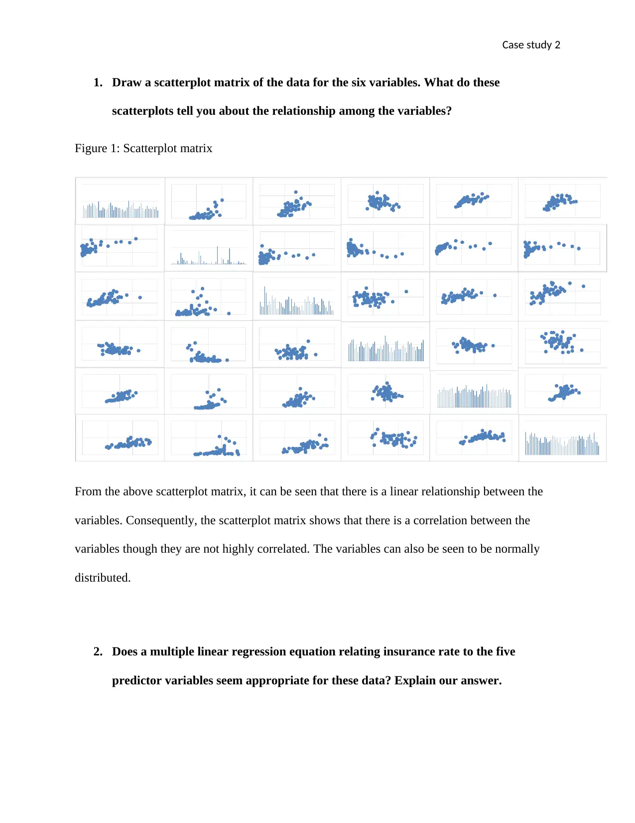
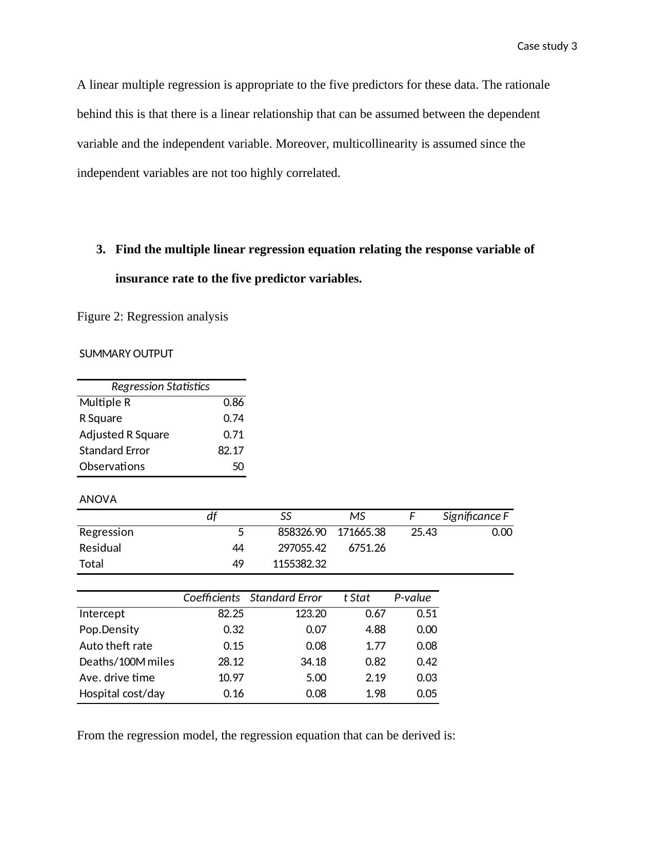
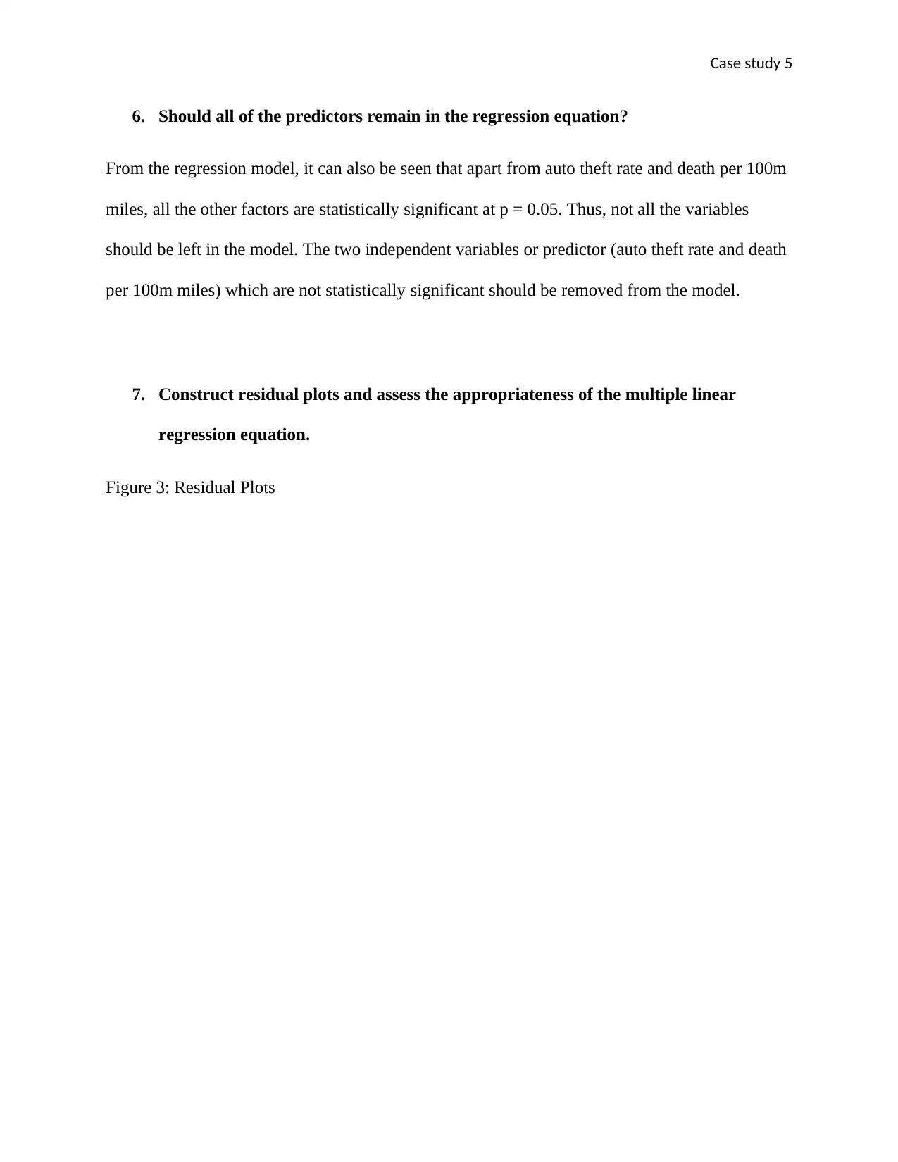
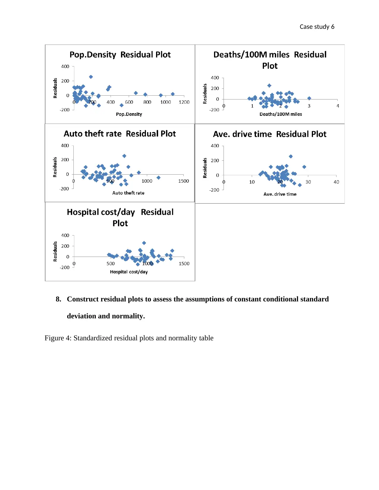
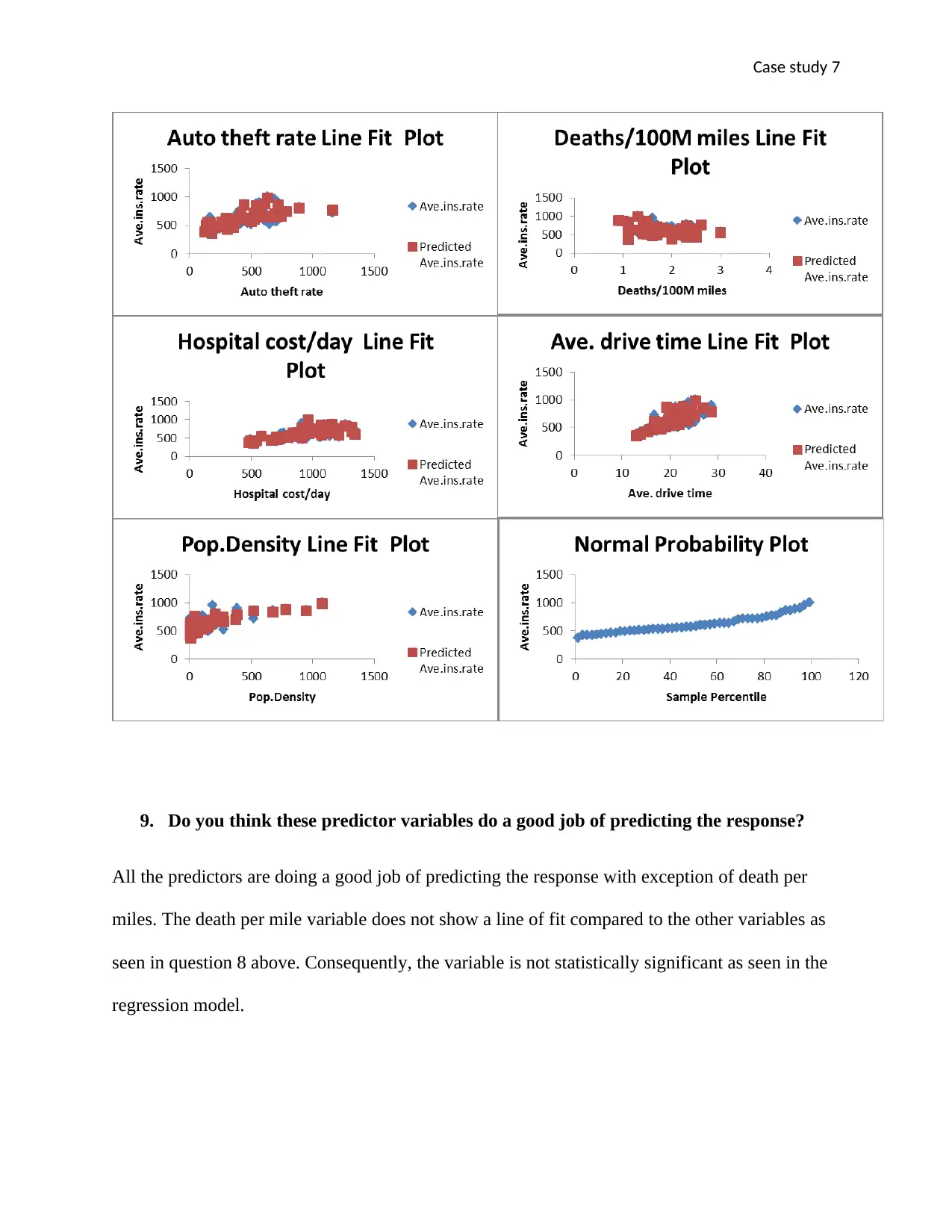
This case study utilizes multiple linear regression to analyze the factors influencing insurance rates. A scatterplot matrix reveals linear relationships between variables, suggesting the appropriateness of a multiple linear regression model. The derived regression equation, Ave.ins.rate = 82.25 + 0.32Pop.Density + 0.15Auto_theft_rate + 28.12Deaths/100M_Miles + 10.97Ave.drive_time + 0.16Hopsital_cost/day, indicates the impact of each predictor variable on the average insurance rate. The adjusted R-squared value of 0.71 signifies that 71% of the variability in insurance rates is explained by the model's variables. However, statistical significance tests suggest that not all predictors should remain in the equation, specifically auto theft rate and deaths per 100m miles. Residual plots are constructed to assess the model's assumptions and appropriateness, revealing that most predictors perform well in predicting the response variable, except for death per miles. Desklib provides this and other solved assignments to aid students in their studies.

Running Header: Case Study 1
Case Study
Student’s name: Obaid Alshaali
Student’s ID:
Institution:

Case study 2
1. Draw a scatterplot matrix of the data for the six variables. What do these
scatterplots tell you about the relationship among the variables?
Figure 1: Scatterplot matrix
From the above scatterplot matrix, it can be seen that there is a linear relationship between the
variables. Consequently, the scatterplot matrix shows that there is a correlation between the
variables though they are not highly correlated. The variables can also be seen to be normally
distributed.
2. Does a multiple linear regression equation relating insurance rate to the five
predictor variables seem appropriate for these data? Explain our answer.

Case study 3
A linear multiple regression is appropriate to the five predictors for these data. The rationale
behind this is that there is a linear relationship that can be assumed between the dependent
variable and the independent variable. Moreover, multicollinearity is assumed since the
independent variables are not too highly correlated.
3. Find the multiple linear regression equation relating the response variable of
insurance rate to the five predictor variables.
Figure 2: Regression analysis
SUMMARY OUTPUT
Regression Statistics
Multiple R 0.86
R Square 0.74
Adjusted R Square 0.71
Standard Error 82.17
Observations 50
ANOVA
df SS MS F Significance F
Regression 5 858326.90 171665.38 25.43 0.00
Residual 44 297055.42 6751.26
Total 49 1155382.32
Coefficients Standard Error t Stat P-value
Intercept 82.25 123.20 0.67 0.51
Pop.Density 0.32 0.07 4.88 0.00
Auto theft rate 0.15 0.08 1.77 0.08
Deaths/100M miles 28.12 34.18 0.82 0.42
Ave. drive time 10.97 5.00 2.19 0.03
Hospital cost/day 0.16 0.08 1.98 0.05
From the regression model, the regression equation that can be derived is:

Case study 4
Ave.ins.rate = 82.25 + 0.32Pop.Density + 0.15Auto_theft_rate + 28.12Deaths/100M_Miles +
10.97Ave.drive_time + 0.16Hopsital_cost/day
4. Interpret the sample regression coefficients
From the regression equation, it is evident that the base average insurance rate is 82.25, holding
all factors constant. On the other hand, a unit increase in population density increases the average
insurance rate by 0.32 units holding all factors constant. Similarly, auto theft rate, deaths per
100m miles, average drive time, and hospital cost per day increases the average insurance rate by
0.15, 28.12, 10.97, and 0.16 units apiece. All the factors have to be kept constant for each
variable.
Moreover, all the variables are statistically significant with exception to the intercept, auto theft
rate and deaths per 100 miles at p = 0.05.
5. Determine the proportion of variation in the observed insurance rates that can be
accounted for by the multiple linear regression equation in the five predictor
variables.
From the regression statistics, it is seen that the value of the adjusted R squared is 0.71. Thus,
71% of the variability in the regression model is explained by factors in the model that is the five
independent variables. However, 29% of the variability is explained by variables or factors
which are not in the model.

Case study 5
6. Should all of the predictors remain in the regression equation?
From the regression model, it can also be seen that apart from auto theft rate and death per 100m
miles, all the other factors are statistically significant at p = 0.05. Thus, not all the variables
should be left in the model. The two independent variables or predictor (auto theft rate and death
per 100m miles) which are not statistically significant should be removed from the model.
7. Construct residual plots and assess the appropriateness of the multiple linear
regression equation.
Figure 3: Residual Plots

Case study 6
8. Construct residual plots to assess the assumptions of constant conditional standard
deviation and normality.
Figure 4: Standardized residual plots and normality table

Case study 7
9. Do you think these predictor variables do a good job of predicting the response?
All the predictors are doing a good job of predicting the response with exception of death per
miles. The death per mile variable does not show a line of fit compared to the other variables as
seen in question 8 above. Consequently, the variable is not statistically significant as seen in the
regression model.