Intermediate Economics Assignment: Utility and Budget Constraints
VerifiedAdded on 2019/11/20
|10
|1259
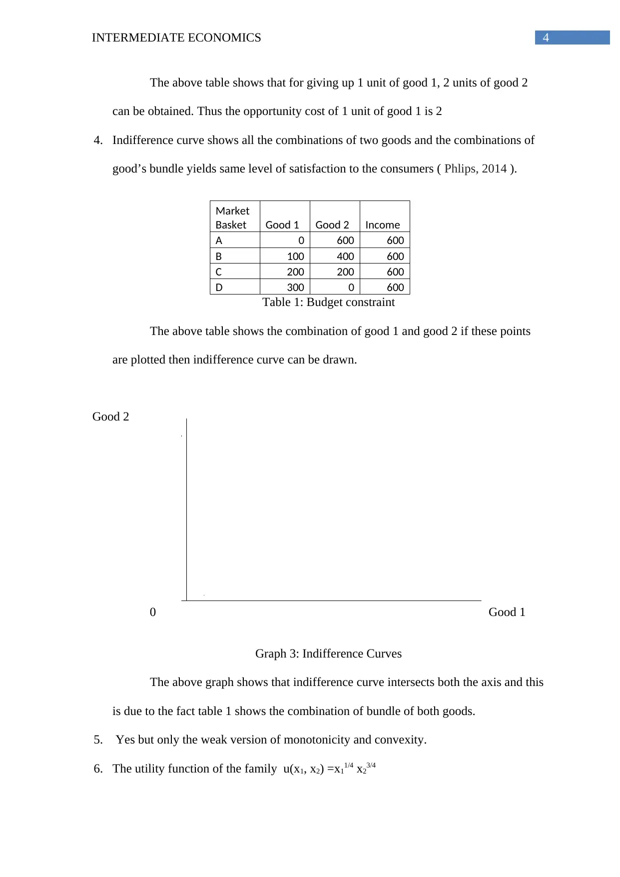
|320
Homework Assignment
AI Summary
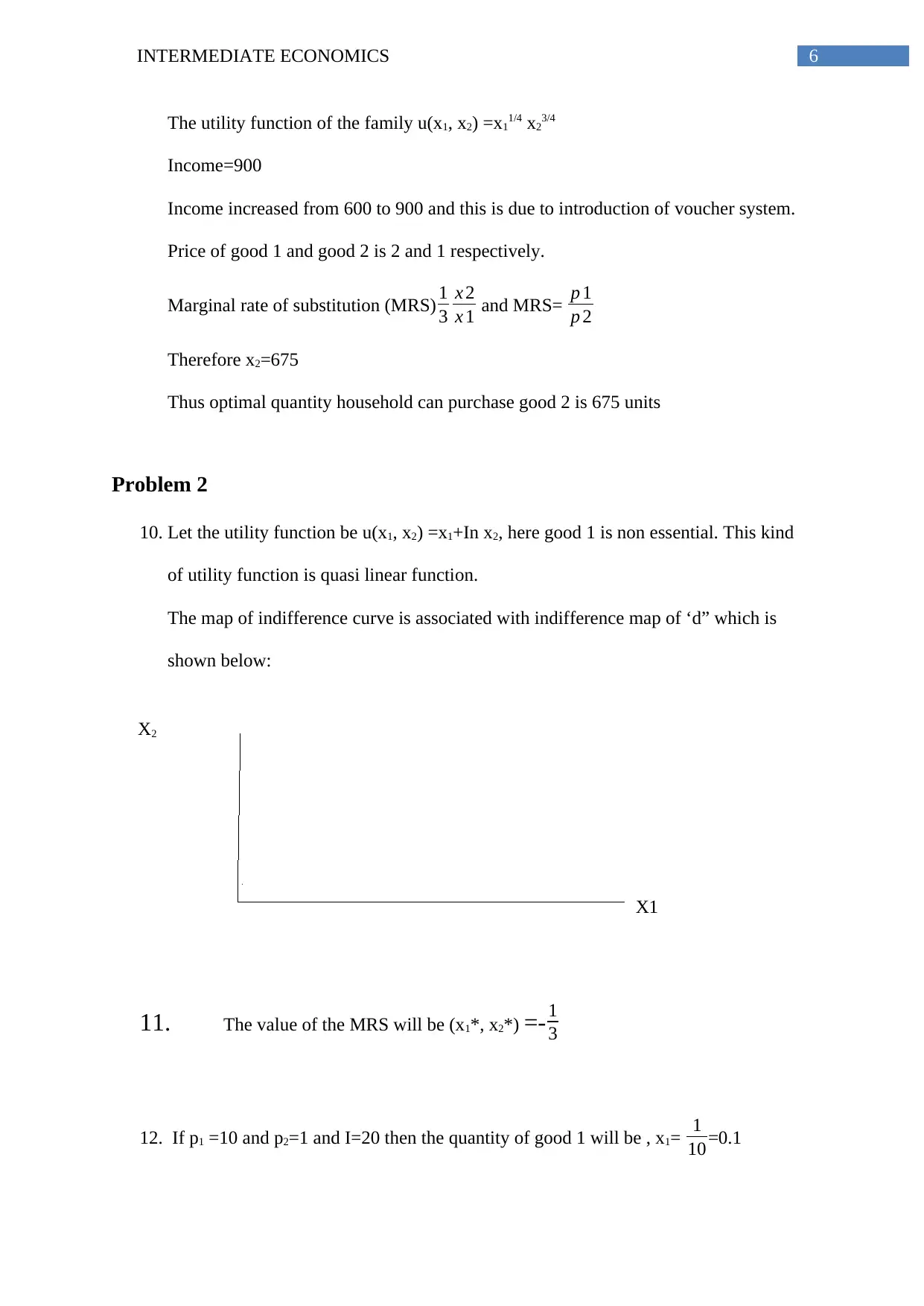
This economics assignment delves into consumer behavior, analyzing how individuals make choices within budget constraints and maximize utility. Problem 1 examines a family's consumption of two goods, exploring budget lines, indifference curves, and the impact of a voucher system on optimal consumption. Problem 2 introduces a quasi-linear utility function, investigating the marginal rate of substitution and consumer choices with varying incomes and prices. Problem 3 focuses on a utility function with perfect substitutes, assessing the effects of price changes on consumer behavior, substitution, and income effects, and identifying whether goods are Giffen or normal. The assignment utilizes graphs, tables, and mathematical calculations to illustrate economic principles and provide detailed solutions to each problem.
1 out of 10
Related Documents


Your All-in-One AI-Powered Toolkit for Academic Success.
+13062052269
info@desklib.com
Available 24*7 on WhatsApp / Email
![[object Object]](/_next/static/media/star-bottom.7253800d.svg)
Copyright © 2020–2026 A2Z Services. All Rights Reserved. Developed and managed by ZUCOL.