EC206: Intermediate Mathematics for Economics - Assignment Solution

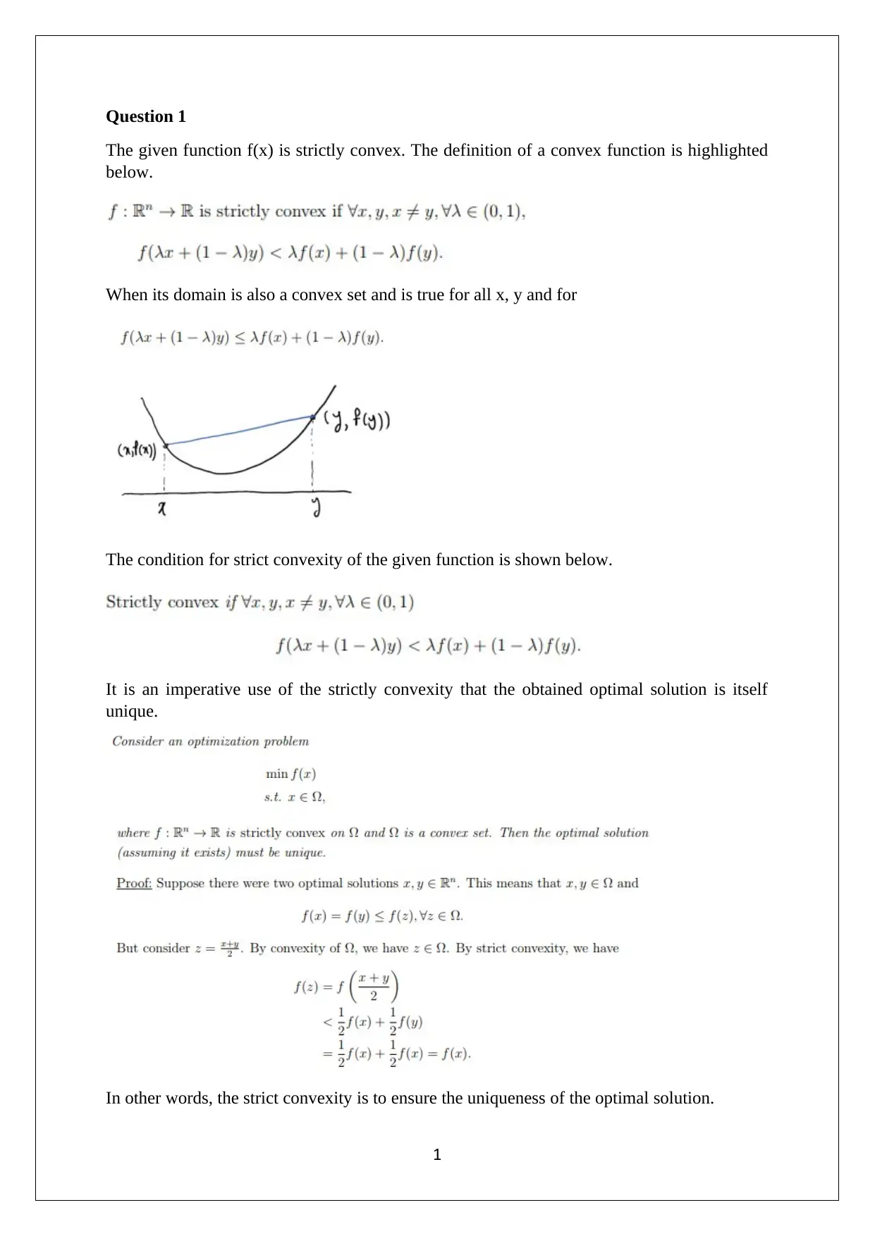
This document presents a comprehensive solution to the EC206 Intermediate Mathematics for Economics assignment. The solution addresses several key areas, including the concept of convexity, discussing its properties and implications for optimization, supported by a diagram. It then delves into calculus, providing detailed calculations of partial and total derivatives for various functions, simplifying expressions where possible. The solution further explores symmetric functions, demonstrating how arguments can be swapped without changing the function's outcome. Additionally, it analyzes production functions, calculating the marginal rate of technical substitution and deriving isoquant equations. Finally, the document tackles optimization problems using the Lagrangian method, determining first-order conditions, solving for optimal values, and demonstrating the solution's maximum properties through second-order derivative analysis. The solution is a thorough guide for students studying intermediate mathematics for economics.

EC206 Intermediate Mathematics for Economics
[Document subtitle]
[DATE]

Question 1
The given function f(x) is strictly convex. The definition of a convex function is highlighted
below.
When its domain is also a convex set and is true for all x, y and for
The condition for strict convexity of the given function is shown below.
It is an imperative use of the strictly convexity that the obtained optimal solution is itself
unique.
In other words, the strict convexity is to ensure the uniqueness of the optimal solution.
1

Question 2
(a) Partial and total derivative of z with respective to x and y
z=ln ( x2 y )
x + y=1
Partial derivative of z with respect to x
∂ z
∂ x = ∂ ln ( x2 y )
∂ x
Let u=x2 y
∂ z
∂ x = ∂ ln ( u )
∂ x . ∂ ( x2 y )
∂ x
∂ z
∂ x = 1
u∗2 y∗x2 y−1= 1
x2 y ∗2 y x2 y−1=2 y x2 y−1+2 y =2 y x−1= 2 y
x
Now ,
With respect to y
∂ z
∂ y = ∂ ln ( x2 y )
∂ y
Let u=x2 y
∂ z
∂ y = ∂ ln ( u )
∂ y . ∂ ( x2 y )
∂ y
From exponent rule: x2 y=e2 yln(x)
∂ z
∂ y = ∂ ln ( u )
∂ y . ∂ ( e2 yln (x ) )
∂ y =1
u .2 x2 y ln ( x )
∂ z
∂ y = 1
x2 y . 2 x2 y ln ( x ) =1.2 ln ( x )=2 ln (x )
Hence, the partial derivatives would be 2 y
x ,2 ln (x)
Total derivative of z
dz= ∂ z
∂ x dx + ∂ z
∂ y dy
dz= 2 y
x dx +2 ln( x )dy
Here,
x + y=1
2

dx +dy =0
dy =−dx
Thus,
dz= 2 y
x dx +2 ln ( x ) (−dx )
dz= ( 2 y
x −2 ln ( x ) )dx
dz= 2
x ( y −x ln ( x ) ) dx
(b) Partial and total derivative of z with respective to x and y
z=x + y
A xa yb =k
Where, a , b∧k are constants
Partial derivative of z with respect to x
∂ z
∂ x = ∂(x + y )
∂ x =1
With respect to y
∂ z
∂ y = ∂( x+ y )
∂ y =1
Total derivative of z
dz= ∂ z
∂ x dx + ∂ z
∂ y dy
Divide by dx
dz
dx = ∂ z
∂ x + ∂ z
∂ y
dy
dx
dz
dx =1+1. dy
dx
Now,
A xa yb =k
x= ( k
y b A )1
a
Similarly,
3

y= ( k
xa A )1
b
dz
dx =1+1.
d ( ( k
xa A ) 1
b
)
dx =1+ d
dx ( k
1
b
x
a
b . A
1
b )
dz
dx =1+ ( k
A )1
b
( d
dx (x
a
b ) )=1+ ( k
A )1
b
( a
b )x− ( a
b +1 )
Further,
dz= ∂ z
∂ x dx + ∂ z
∂ y dy
Divide by dy
dz
dy = ∂ z
∂ y + ∂ z
∂ x
dx
dy
dz
dy =1+1. dx
dy
dz
dy =1+1.
d ( ( k
yb A ) 1
a
)
dy =1+ d
dy ( k
1
a
y
b
a . A
1
a ) =1+ ( k
A ) 1
a
( d
dx ( y
−b
a ) )=1− ( k
A ) 1
a
( b
a ) y−( b
a +1 )
Question 3
(a) The given function would be termed as symmetric in its arguments when the reversal of
the arguments would not make any change in the function.
z=f (x1 , x2)
z= A (∝1 x1
−β +∝2 x2
−β )−1
β
Where, A>0 ,∝>0 , i=1 , 2∧β >−1
Swapping of the arguments
Original: z=f (x1 , x2)=A ( ∝1 x1
− β +∝2 x2
− β ) −1
β
Swapping: z=f (x2 , x1)=A ( ∝1 x2
− β +∝2 x1
− β ) −1
β
It is apparent that ∝1∧∝2are constant and hence, can be assumed to be equal ∝1=∝2
4

Therefore, it can be concluded that swapping of the arguments would not change the original
function.
z=f ( x1 , x2)=f (x2 , x1 )
(b)
(i) ∂ z
∂ x1
Function of x1 for x2
∂ z
∂ x1
= ∂
∂ x1
{ A ( ∝1 x1
− β +∝2 x2
− β
)
−1
β }
∂ z
∂ x1
= A ( −1
β ) ( ∝1 x1
−β +∝2 x2
−β ) −1
β −1 ∂
∂ x1
( ∝1 x1
− β +∝2 x2
− β )
∂ z
∂ x1
= A ( −1
β ) ( ∝1 x1
−β +∝2 x2
−β ) −1
β −1
. ∝1 ( −β ) x1
−β −1
∂ z
∂ x1
= A ( −1
β ) ( −β ) ( ∝1 x1
− β +∝2 x2
− β ) −1
β −1
. ∝1 x1
−β −1
∂ z
∂ x1
= A ∝1 x1
− β−1 ( ∝1 x1
− β +∝2 x2
− β )−1
β −1
(ii) ∂ z
∂ x1
Function of x1 for x2
∂ z
∂ x1
= A ∝1 x1
− β−1 ( ∝1 x1
− β +∝2 x2
− β )−1
β −1
The given function is symmetric in its arguments when the reversal of the arguments has not
made any change in the function.
z=f ( x1 , x2)=f (x2 , x1 )
Thus,
Function of x1 for x2
∂ z
∂ x2
= A ∝1 x2
− β−1 ( ∝1 x1
− β +∝2 x2
− β )−1
β −1
5

(c) ∂ z
∂ x1
i=1 , 2
x1
∂ z
∂ x1
+ x2
∂ z
∂ x2
=z
Here, put the values of
∂ z
∂ x1
∧∂ z
∂ x2
in the above function
LHS ¿ x1
∂ z
∂ x1
+ x2
∂ z
∂ x2
¿ x1 . {A ∝1 x1
−β−1
(∝1 x1
− β +∝2 x2
− β
)−1
β −1
}+ x2 . {A ∝2 x2
−β−1
(∝1 x1
− β +∝2 x2
− β
)−1
β −1
}
¿ A (∝1 x1
−β +∝2 x2
−β )−1
β −1
(∝1 x1
−β −1 . x1+∝2 x2
−β −1 x2)
¿ A (∝1 x1
−β +∝2 x2
−β )−1
β −1
(∝1 x1
−β −1+1 +∝2 x2
− β−1+1 )
¿ A (∝1 x1
−β +∝2 x2
−β )−1
β −1
(∝1 x1
−β + ∝2 x2
−β )
¿ A (∝1 x1
−β +∝2 x2
−β )−1
β −1+1
¿ A (∝1 x1
−β +∝2 x2
−β )−1
β
¿ z
RHS = z
Hence, proved LHS =RHS
x1
∂ z
∂ x1
+ x2
∂ z
∂ x2
=z
(d) Euler’s theorem holds this function or not?
It can be seen that the degree of the function is 1.
Hence,
∑
i=1
2
xi
df
d xi
=z=f
The function holds Euler’s theorem.
6

Question 4
(a) Production function
Q=a ln ( x1 )+ b ln(¿ x2)¿
Where, a , b=Positive numbers, x1∧x2=Quantity inputs
Marginal rate expression
Total derivative of output Q w. r. t. x1
dQ
d x1
= d
d x1
¿
Total derivative of output Q w. r. t. x2
dQ
d x2
= d
d x2
¿
Hence, Marginal rate of technical substitution=
a
x1
b
x2
= a x2
b x1
(b) Equation of an isoquant x2 for a fixed Q in terms of x1
¿
ln ( x1
a ) +ln (¿ x2
b )=Q ¿
ln (¿ x2
b )=Q−ln ( x1
a ) ¿
Take the exponential of both the sides
x2
b=eQ −x1
a
x2=¿ ¿
Equation of an isoquant x2 for a fixed Q in terms of x1 would be x2=¿ ¿
(c) Marginal rate of technical substitution of x1for x2 , for x2 not in terms of Q and hence, first
task is to eliminate Q
Expression from part b
x2=¿ ¿
Here,
x2
b=eQ −x1
a
7

eQ=x2
b + x1
a
Take natural log
Q=ln ¿ ¿
Q=ln( x2
b∗x1
a )
Now, Again
eQ=x2
b∗x1
a
Substitute the eQ=x2
b∗x1
a in eq. 1
x2=¿
x2={x1
a
( x2
b – 1 ) }
1
b
x2= ( x1
a
b ) { ( x2
b – 1 ) }
1
b
Now,
∆ x2
∆ x1
= ∆
∆ x1
(x1
a
b ){( x2
b – 1 ) }
1
b
∆ x2
∆ x1
={( x2
b – 1 ) }
1
b
( a
b ) ( x1
a
b −1
)
∆ x2
∆ x1
={( x2
b – 1 ) }
1
b
( a
b ) ( x1
a−b
b )
∆ x2
∆ x1
= {( x2 ) ( a
b ) ( x1
a ) ( x1
−1 ) }= ( a
b ) ( x2
x1 )x1
a
Or
∆ x2
∆ x1
= ( a
b ) ( x2
x1 )
Question 5
(a) The aim of the manager is to maximize the profit (π )
x , y are the outputs of the two products manufactured by the fir,
Profit function
Maximize π=50 x−2 x2−xy−3 y2 +95 y
x + y=25
8

Lagrangean for the given case to show the Lagrange multiplier
∂
∂ x ∅ =π + λ ( 25−x− y )
∂∅
∂ x = ∂
∂ x { ( 50 x−2 x2−xy−3 y2 +95 y ) + λ ( 25−x− y ) }
(b) First order conditions
∂∅
∂ x = ∂
∂ x { ( 50 x−2 x2−xy−3 y2 +95 y ) + λ ( 25−x− y ) }
∂∅
∂ x =50−4 x− y−0+ 0+ ( −λ )
∂∅
∂ x =50−4 x− y−λ
Put ∂∅
∂ x =0
50−4 x− y −λ=0 … … … … ( 1 )
Now,
∂∅
∂ y = ∂
∂ y { ( 50 x−2 x2−xy−3 y2 +95 y ) + λ ( 25−x− y ) }
∂∅
∂ y =−x −6 y+ 95+ (−λ )
Put
∂∅
∂ y =0
∂∅
∂ y =95−6 y −x−λ … … … ..(2)
Similarly,
∂∅
∂ λ = ∂
∂ λ { ( 50 x−2 x2 −xy−3 y2+ 95 y ) + λ ( 25−x− y ) }
Put
∂∅
∂ λ =0
∂∅
∂ λ =25−x− y=0 … … … … .(3)
9

(c) Solve the three equation to find the value of first order conditions which is x*, y* λ*
50−4 x− y −λ=95−6 y−x−λ
−45−3 x=−5 y
y=9+( 3
5 ) x
25−x− y=0
25−x− {9+( 3
5 ) x }=0
25−x−9−3
5 x=0
16−8 x
5 =0
80−8 x=0
x=10 or say x∗¿ 10
y=9+( 3
5 ) x +9+ (3
5 )10
y∨ y∗¿ 15
50−4 x− y −λ=0
50−40−15−λ=0
−5−λ=0
λ∗¿−5
Now, profit
π=50 x−2 x2−xy−3 y2 +95 y
π=50∗10−2¿ 102−10∗15−3 152+ 95∗15
π∗¿ 1925−1025=900
(d) Show that the solution is maximum
The first step is to find the second derivative of the function
∂2 L
∂ x2 =0 (For maximization , second order ) (w.r.t.x)
∂2 L
∂ x2 = ∂2
∂ x2 { ( 50 x−2 x2 −xy−3 y2+95 y ) +λ ( 25−x− y ) }
10

¿ ∂
∂ x ¿
¿ ∂
∂ x {50−4 x− y +5 }
¿−4
−4<0
Similarly,
∂2 L
∂ y2 =0( For maximization , second order) (w.r.t.y)
∂2 L
∂ y2 = ∂2
∂ y2 { ( 50 x−2 x2−xy−3 y2 +95 y ) + λ (25−x− y ) }
¿ ∂
∂ y ¿
¿ ∂
∂ y { −x−6 y +95+5 }
¿−6
−6<0
Both,
∂2 L
∂ x2 ∧∂2 L
∂ y2 <0
Hence, it can be sad that the solution is a maximum because the second derivative comes out
to be lower than zero.
(e) Interpretation
50−4 x− y −λ=0
50−40−15−λ=0
−5−λ=0
λ∗¿−5
The economical interpretation of the Lagrange multiplier represents that for a given utility
maximizing problem is the marginal utility of the time. The λ∗¿ indicates the rate of change in the
extreme value with respect to the change in the constraints. The optimal value of the λ∗¿ indicates
the measures of the marginal utility of the income which means the rate of increase in maximized
utility increases as the corresponding income increases.
(f) Approximate change in the maximized profit when the output constraints reduced from 25 to 24.
11