International Business Statistics Report: Data Analysis and Findings

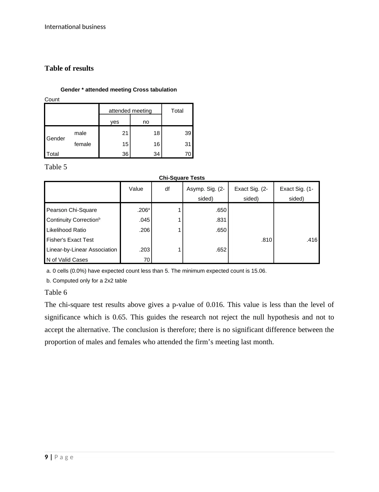
This report presents an analysis of international business statistics, focusing on a research study conducted by a local council regarding the recycling of food waste and the potential of biogas production. The report begins with a data requirement table outlining the research objectives, sampling method (simple random sampling), and data collection tool (semi-structured questionnaire). Part B of the report includes data analysis using histograms, and tables to display findings on employee demographics, income statistics, and the relationship between years worked and salary using linear regression. Furthermore, the report explores the difference in mean salary among different skill categories using ANOVA and Tukey HSD tests. Finally, the report examines the difference between proportions of males and females who attended a firm's meeting using a Chi-square test. The results of these statistical analyses are presented with interpretations, conclusions, and relevant tables. References are also provided.

International business
Statistics
Student name:
Tutor name:
1 | P a g e

International business
PART A
Data requirement table
Table 1 source: Saunders et al, 2012, p. 425
Research purpose
Cooking gas has in the recent past become so expensive that only few households can afford it.
To add on, the gas has not been environmentally friendly due to the carbon particles produced
into the atmosphere. There has been an idea that waste products can be able to be recycled by
way of converting them to biogas fuel. Given that this is an area where food waste is produced
daily in tones, there was need to try the biogas produced by food waste. The local council prior
to venturing into this project thought it wise to collect data on the views of the locals about the
same topic. So a research had to be carried out first. The objective of this research was to gather
information from households regarding the recycling of food waste. The information gathered
then would be used to guide decision making as far as recycling waste food staff and use of
biogas was concerned. The population of the study included all the households within the local
council jurisdiction.
Sampling method
The research study employed the use of simple random sampling to obtain a sample from which
the information is to be collected. Simple random sampling also known as probability sampling
was employed in this case since most of the residents in the local council were using the normal
gas thereby understood or had a feeling of how expensive it was and therefore cases of biasness
were minimized (Boynton 2014). It was also cheaper and less time consuming to apply simple
2 | P a g e

International business
random sampling as compared to methods such as multi-stage sampling. The other reason is that
it gave every household in the local council and equal chance of being selected in the sample
(Dillman 2016). This method also ensured that the sample finally achieved did represent the
entire population without bias. The sample collected thus becomes a representative of the whole
population.
Data collection tool (questionnaire)
The research study decided to use a questionnaire as a tool for data collection. There are three
types of questionnaires; structured questionnaire, unstructured questionnaire and semi-structured
questionnaires (Bradburn 2014). However, the research study decided to a semi-structured
questionnaire. Semi-structured questionnaire was appropriate in this case. This is because a semi-
structured questionnaire is not standardized and always leans much on qualitative research
(Oppenheim 2011). The interviewer is not obliged to strictly follow the set of questions but is
left to use his or her due diligence to ask information that he feels is necessary even if it is not in
the questionnaire but related to a topic in the questionnaire (Foddy 2013). This also gives the
respondents some latitude to air their views, feelings and opinions. This in turn leads to
collection of very rich and insightful information.
Data requirement table
A data requirement table is very important when it comes to preparation for a survey. It gives the
researcher an outline of the not only the objective of the research but also the type of research.
This helps to guide the whole process of conducting the research. It also outlines the questions to
be answered, the type of variable and their levels of measurements.
3 | P a g e

International business
PART B
Histogram showing the distribution of the workforce
Figure 1
The figure above shows the age distribution of the respondents. From the histogram, it can be
observed that the ages were normally distributed. However, at the center, where the people in
middle age are, the frequency was low meaning that the people at this particular age were fewer
compared to the lower age and the older age.
4 | P a g e

International business
Ethnic distribution of employees
Figure 2
Figure 2 above is of distribution of employees according to their ethnic backgrounds. It can be
observed that the white were 36 while the Asians were 18. The West Indians were 14 while the
Africans were only 2. The majority of the employees were the white who constituted to 50% of
all the employees. This was followed by the Asians who constituted to 25% of the total
employees. The other group which was the West Indians constituted to 19.44%. The Africans
constituted to only 2.8% of the total employees.
Average income
Statistics
Income
N Valid 68
Missing 2
Mean 7819.12
Median 7800.00
Std. Deviation 997.947
Variance 995897.717
Minimum 5900
Maximum 10500
5 | P a g e

International business
Table 1
The table above shows the descriptive statistics of the salary of all the employees. It gives both
the measures of center and measures of dispersion. The measure of center was the mean and
median which were 7819.12 and 7800 respectively. The measures of dispersion are the standard
deviation and variance. They are 997.95 and 995,897.72 respectively. The lowest paid employee
earned 5900 while the highest paid employee earned 10500.
The mean income was 7819.12
Relationship between years worked and salary (linear regression)
Model Summary
Model R R Square Adjusted R
Square
Std. Error of the
Estimate
1 .340a .115 .102 945.711
a. Predictors: (Constant), Years Worked
ANOVAa
Model Sum of Squares df Mean Square F Sig.
1
Regression 7696787.937 1 7696787.937 8.606 .005b
Residual 59028359.122 66 894369.078
Total 66725147.059 67
a. Dependent Variable: Income
b. Predictors: (Constant), Years Worked
Table 2
Coefficientsa
Model Unstandardized Coefficients Standardized
Coefficients
t Sig.
B Std. Error Beta
1 (Constant) 7410.810 180.346 41.092 .000
Years Worked 31.841 10.854 .340 2.934 .005
a. Dependent Variable: Income
Table 3
6 | P a g e

International business
Table 2 and 3 shows the results of regression analysis between the age as the independent
variable and salary as the dependent variable. The R-squared value is 0.115 indicating that the
independent variable (years worked) is responsible for the 11.5% variation that occurs in the
dependent variable (salary). The y-intercept is positive meaning that there is a positive
relationship between years worked and salary; an increase in years worked led to an increase in
salary. The beta value for years worked is 31.84 meaning that a unit change in the variable
“years worked” leads to 31.84 units change in amount of salary.
Anova test for the difference in mean salary among different skill categories
Hypothesis
H0: The mean salary is equal among all different skill categories
H1: At least one skill category has got a different mean.
Level of significance = 0.05
Table of results is as below;
ANOVA
Income
Sum of Squares df Mean Square F Sig.
Between Groups 9891797.852 3 3297265.951 3.713 .016
Within Groups 56833349.206 64 888021.081
Total 66725147.059 67
Table 3
The anova results above gives a p-value of 0.016. This value is less than the level of significance
which is 0.05. This guides the research to reject the null hypothesis and accept the alternative.
The conclusion is therefore; at least one skill category has got a different mean. In order to
identify the skills which had significantly different means, a Tukey HSD test was employed and
the results were as seen in the table below.
7 | P a g e

International business
Tukey HSD further test
Income
rated skill N Subset for alpha = 0.05
1 2
Tukey HSDa,b
semi-skilled 18 7288.89
unskilled 14 7628.57 7628.57
fairly skilled 20 8095.00 8095.00
highly skilled 16 8237.50
Sig. .074 .252
Means for groups in homogeneous subsets are displayed.
a. Uses Harmonic Mean Sample Size = 16.703.
b. The group sizes are unequal. The harmonic mean of the group sizes is
used. Type I error levels are not guaranteed.
Table 4
As can be observed, the skills which had salary averages significantly different from the rest
were the semi-skilled employees (7288.89) and highly skilled (8237.5).
Chi-square test for the difference between proportions
Is there a significant difference between the proportion of males and females who attended the
firm’s meeting last month?
Hypothesis
H0: There is no significant difference between the proportion of males and females who attended
the firm’s meeting last month.
H1: There is a significant difference between the proportion of males and females who attended
the firm’s meeting last month.
Level of significance = 0.05
8 | P a g e

International business
Table of results
Gender * attended meeting Cross tabulation
Count
attended meeting Total
yes no
Gender male 21 18 39
female 15 16 31
Total 36 34 70
Table 5
Chi-Square Tests
Value df Asymp. Sig. (2-
sided)
Exact Sig. (2-
sided)
Exact Sig. (1-
sided)
Pearson Chi-Square .206a 1 .650
Continuity Correctionb .045 1 .831
Likelihood Ratio .206 1 .650
Fisher's Exact Test .810 .416
Linear-by-Linear Association .203 1 .652
N of Valid Cases 70
a. 0 cells (0.0%) have expected count less than 5. The minimum expected count is 15.06.
b. Computed only for a 2x2 table
Table 6
The chi-square test results above gives a p-value of 0.016. This value is less than the level of
significance which is 0.65. This guides the research not reject the null hypothesis and not to
accept the alternative. The conclusion is therefore; there is no significant difference between the
proportion of males and females who attended the firm’s meeting last month.
9 | P a g e

International business
References
Boynton PM, Greenhalgh T. Selecting, designing and developing your Questionnaire. BMJ,
328:1312- 15, 2014.
Bradburn. Asking Questions: The definitive guide to Questionnaire design. Wiley, 2014.
Dillman DA. Mail and Internet Surveys: The Tailored Design Method. Wiley & Sons, 2016.
Foddy W Constructing Questions for Interviews and Questionnaires: Theory and Practice in
Social Research Cambridge University Press, 2013.
Oppenheim A. Questionnaire Design, Interviewing and Attitude Measurement. London: Pinter
Publishers Ltd, 2011.
10 | P a g e