LCBB6002: International Financial Management - Assessment 2 Analysis

This assignment on International Financial Management (IFM) analyzes investment decision-making using Net Present Value (NPV) and Internal Rate of Return (IRR) methods. It includes calculations of NPV, standard deviation, and expected values for various projects under different scenarios. The assignment evaluates the profitability of projects, compares the NPV and IRR techniques, and determines optimal capital allocation to maximize returns. The analysis covers initial investments, cash flow projections, risk assessments, and the probability of achieving specific financial outcomes. The document provides detailed calculations, rankings of projects, and justifications for investment choices, offering a comprehensive understanding of financial management principles and practical applications.

INTERNATIONAL
FINANCIAL
MANAGEMENT
[ASSESSMENT 2]
1

Table of Contents
Table of Contents.............................................................................................................................2
INTRODUCTION...........................................................................................................................3
MAIN BODY..................................................................................................................................3
Question: 1.......................................................................................................................................3
Question: 2.......................................................................................................................................5
Question: 3.......................................................................................................................................8
a) Calculation of Net Present Value of four projects...................................................................8
b) Reasons for regarding Net Present Value technique superior to internal rate of Return while
project appraisal...........................................................................................................................9
c) Allocation of funds for achieving optimum return in terms of getting highest Net Present
Value..........................................................................................................................................10
CONCLUSION..............................................................................................................................14
REFERENCES..............................................................................................................................15
2

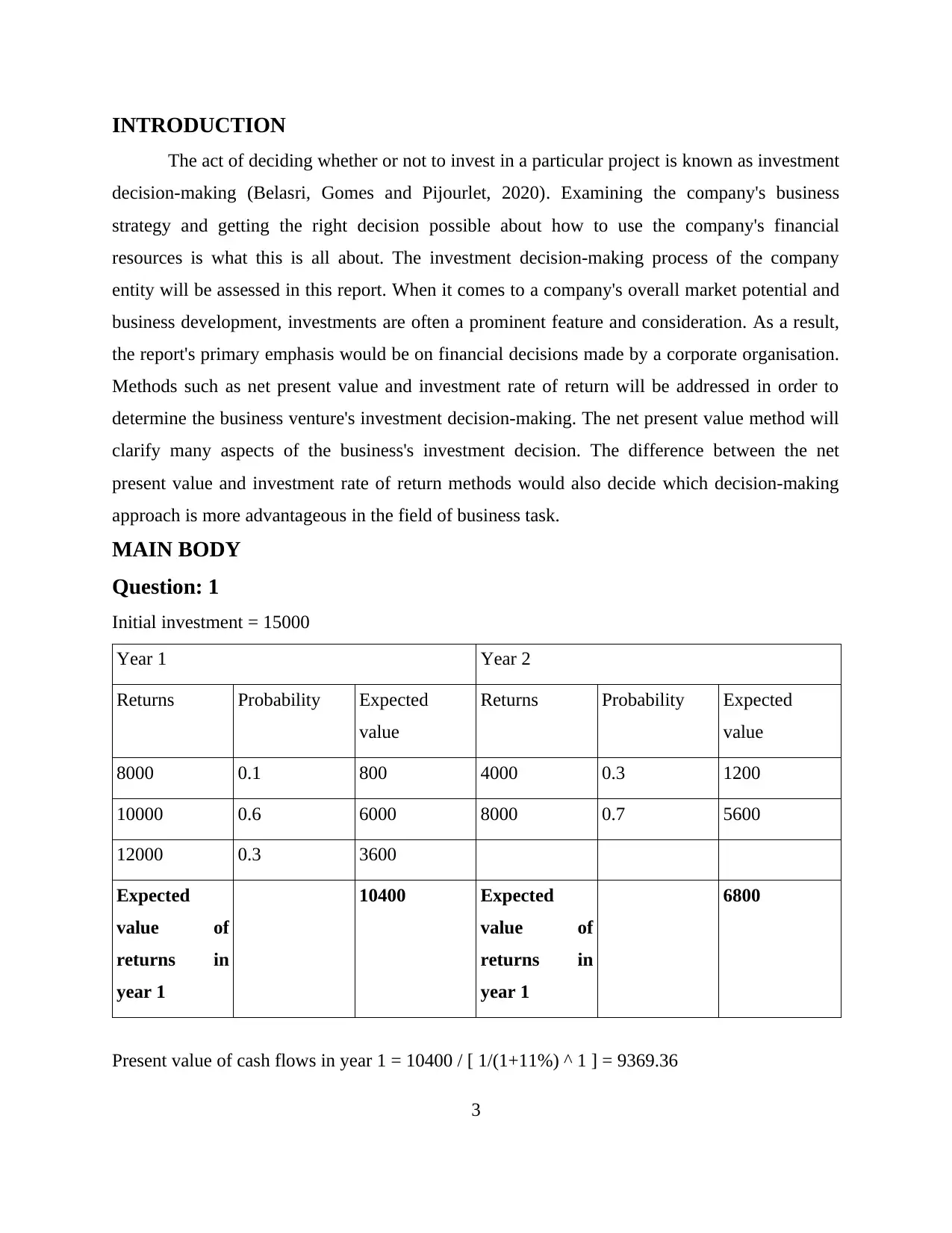
INTRODUCTION
The act of deciding whether or not to invest in a particular project is known as investment
decision-making (Belasri, Gomes and Pijourlet, 2020). Examining the company's business
strategy and getting the right decision possible about how to use the company's financial
resources is what this is all about. The investment decision-making process of the company
entity will be assessed in this report. When it comes to a company's overall market potential and
business development, investments are often a prominent feature and consideration. As a result,
the report's primary emphasis would be on financial decisions made by a corporate organisation.
Methods such as net present value and investment rate of return will be addressed in order to
determine the business venture's investment decision-making. The net present value method will
clarify many aspects of the business's investment decision. The difference between the net
present value and investment rate of return methods would also decide which decision-making
approach is more advantageous in the field of business task.
MAIN BODY
Question: 1
Initial investment = 15000
Year 1 Year 2
Returns Probability Expected
value
Returns Probability Expected
value
8000 0.1 800 4000 0.3 1200
10000 0.6 6000 8000 0.7 5600
12000 0.3 3600
Expected
value of
returns in
year 1
10400 Expected
value of
returns in
year 1
6800
Present value of cash flows in year 1 = 10400 / [ 1/(1+11%) ^ 1 ] = 9369.36
3

Present Value of cash flows in year 2 = 6800 / [ 1/(1+11%) ^ 2 ] = 5521.6
Present value of cash inflows = 14891
a) Net present value of the project = present value of cash inflows – initial investment = (109).
Thus, if the program's net present value (NPV) is negative, that ensures that the project
will result in a net loss for the company, and the company will not continue the project because it
does not appear to be competitive in today's market, according to the current rules of NPV. A
significant reduction in the expected value of the proposal's returns compared to year 1 may be
the reason for the project's negative net present value. The business company will now gain
capital appreciation by investing in the new project as a result of the current project. It is
important in the sense of each project that the business entity earns a higher return on its initial
investment (De Smet, Mention and Torkkeli, 2016). The net present value strategy's basic
premise is that the project's total future inflow must exceed the project's total expenditure. The
above results clearly demonstrate that at this stage of the project's growth, the business enterprise
is incapable of achieving a positive npv outcome.
The company expects to lose money in the second year due to lower inflow, as seen in
the graph above. Since the first year's inflow was so high, the second year's inflow could be half
as high. All of this suggests that the business would lose money on the project. Negative present
value is a weakness in the project because it basically means that if the company invests in it, it
will lose money when it is finished (Duque-Grisales and Aguilera-Caracuel, 2019).
b) The standard deviation of NPV
Year 1
Returns
(X)
D = (X –
Expected value)
D2 Probability Probability * D2
8000 -2400 5760000 0.1 576000
10000 -400 160000 0.6 96000
12000 1600 2560000 0.3 768000
Variance of returns in year 1 = σ2 1440000
4

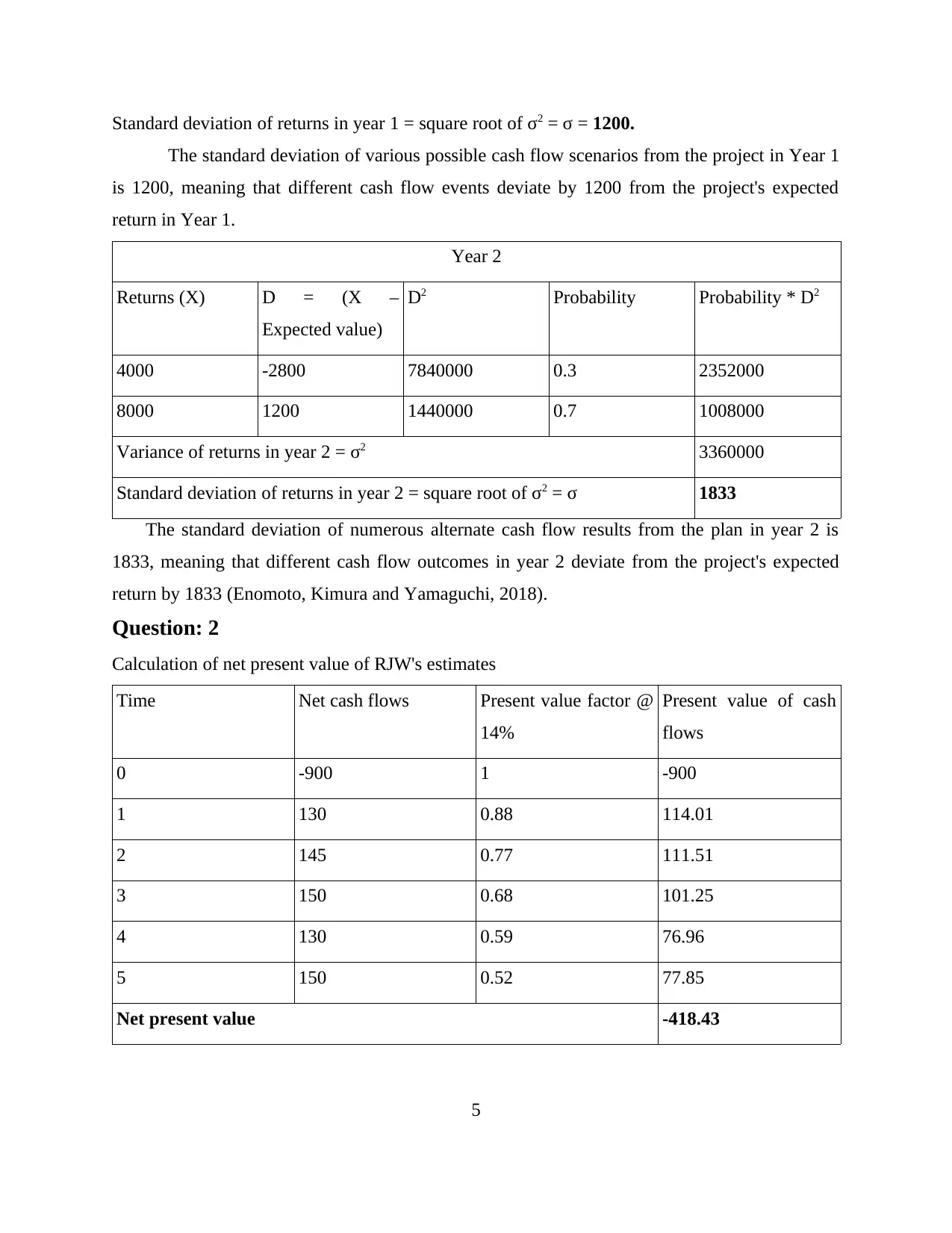
Standard deviation of returns in year 1 = square root of σ2 = σ = 1200.
The standard deviation of various possible cash flow scenarios from the project in Year 1
is 1200, meaning that different cash flow events deviate by 1200 from the project's expected
return in Year 1.
Year 2
Returns (X) D = (X –
Expected value)
D2 Probability Probability * D2
4000 -2800 7840000 0.3 2352000
8000 1200 1440000 0.7 1008000
Variance of returns in year 2 = σ2 3360000
Standard deviation of returns in year 2 = square root of σ2 = σ 1833
The standard deviation of numerous alternate cash flow results from the plan in year 2 is
1833, meaning that different cash flow outcomes in year 2 deviate from the project's expected
return by 1833 (Enomoto, Kimura and Yamaguchi, 2018).
Question: 2
Calculation of net present value of RJW's estimates
Time Net cash flows Present value factor @
14%
Present value of cash
flows
0 -900 1 -900
1 130 0.88 114.01
2 145 0.77 111.51
3 150 0.68 101.25
4 130 0.59 76.96
5 150 0.52 77.85
Net present value -418.43
5

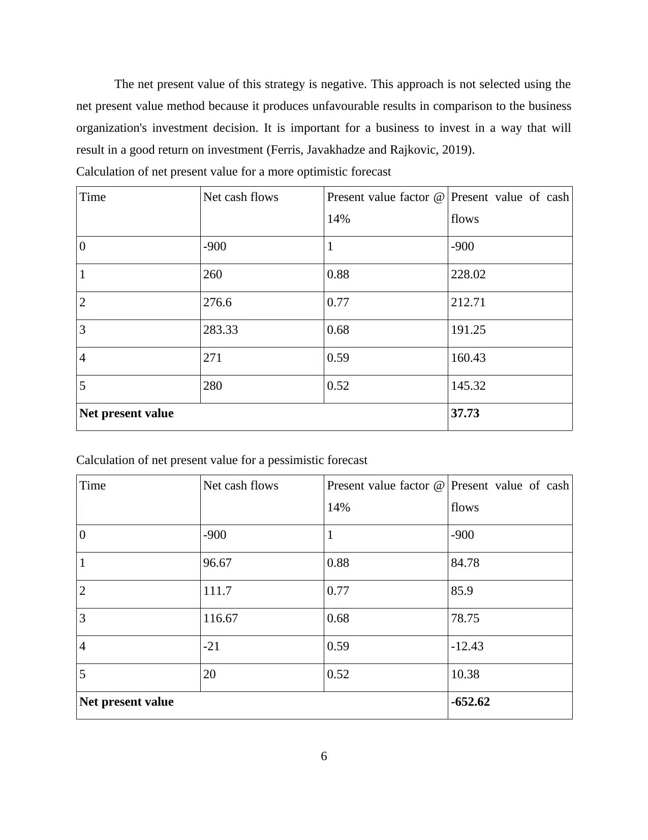
The net present value of this strategy is negative. This approach is not selected using the
net present value method because it produces unfavourable results in comparison to the business
organization's investment decision. It is important for a business to invest in a way that will
result in a good return on investment (Ferris, Javakhadze and Rajkovic, 2019).
Calculation of net present value for a more optimistic forecast
Time Net cash flows Present value factor @
14%
Present value of cash
flows
0 -900 1 -900
1 260 0.88 228.02
2 276.6 0.77 212.71
3 283.33 0.68 191.25
4 271 0.59 160.43
5 280 0.52 145.32
Net present value 37.73
Calculation of net present value for a pessimistic forecast
Time Net cash flows Present value factor @
14%
Present value of cash
flows
0 -900 1 -900
1 96.67 0.88 84.78
2 111.7 0.77 85.9
3 116.67 0.68 78.75
4 -21 0.59 -12.43
5 20 0.52 10.38
Net present value -652.62
6

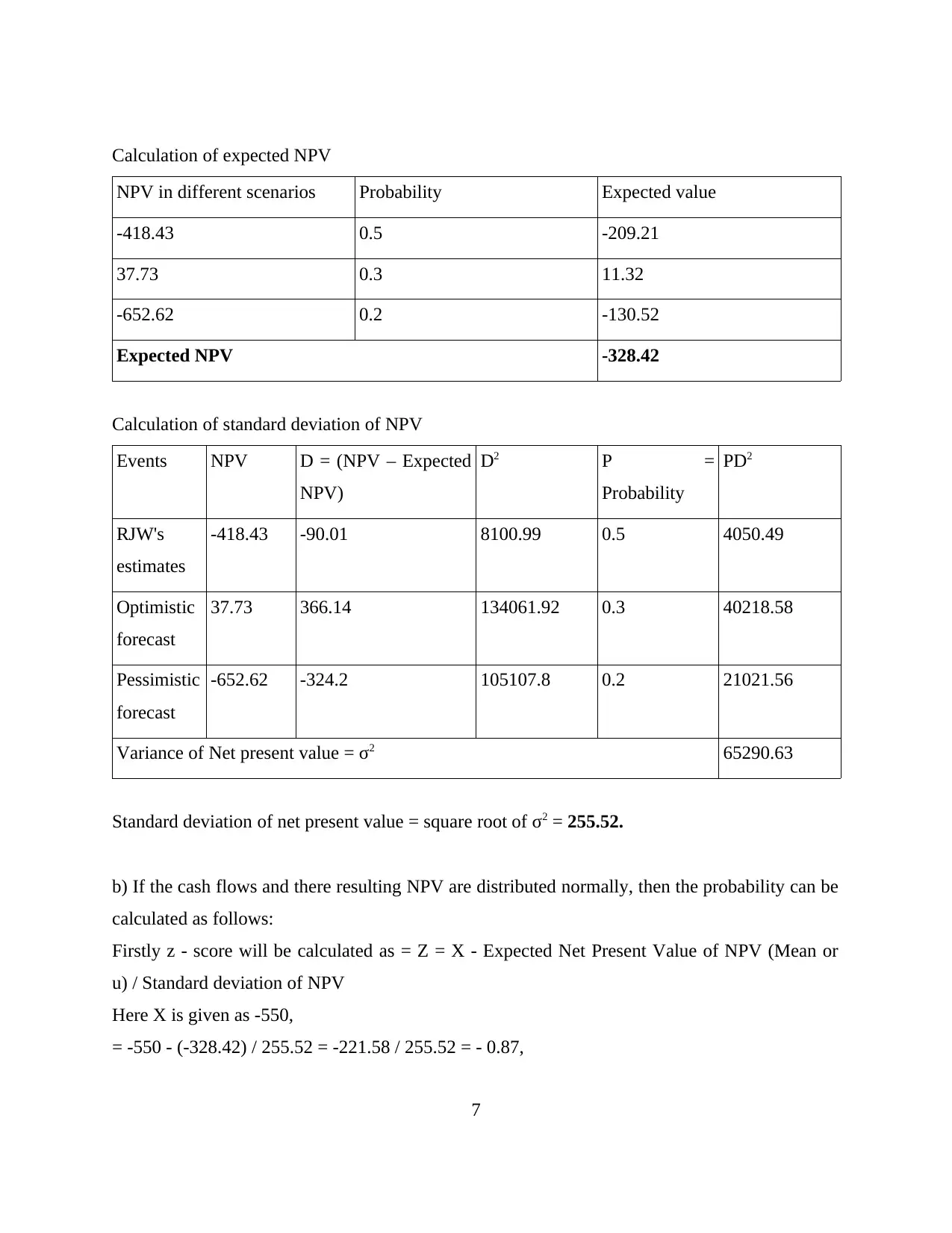
Calculation of expected NPV
NPV in different scenarios Probability Expected value
-418.43 0.5 -209.21
37.73 0.3 11.32
-652.62 0.2 -130.52
Expected NPV -328.42
Calculation of standard deviation of NPV
Events NPV D = (NPV – Expected
NPV)
D2 P =
Probability
PD2
RJW's
estimates
-418.43 -90.01 8100.99 0.5 4050.49
Optimistic
forecast
37.73 366.14 134061.92 0.3 40218.58
Pessimistic
forecast
-652.62 -324.2 105107.8 0.2 21021.56
Variance of Net present value = σ2 65290.63
Standard deviation of net present value = square root of σ2 = 255.52.
b) If the cash flows and there resulting NPV are distributed normally, then the probability can be
calculated as follows:
Firstly z - score will be calculated as = Z = X - Expected Net Present Value of NPV (Mean or
u) / Standard deviation of NPV
Here X is given as -550,
= -550 - (-328.42) / 255.52 = -221.58 / 255.52 = - 0.87,
7

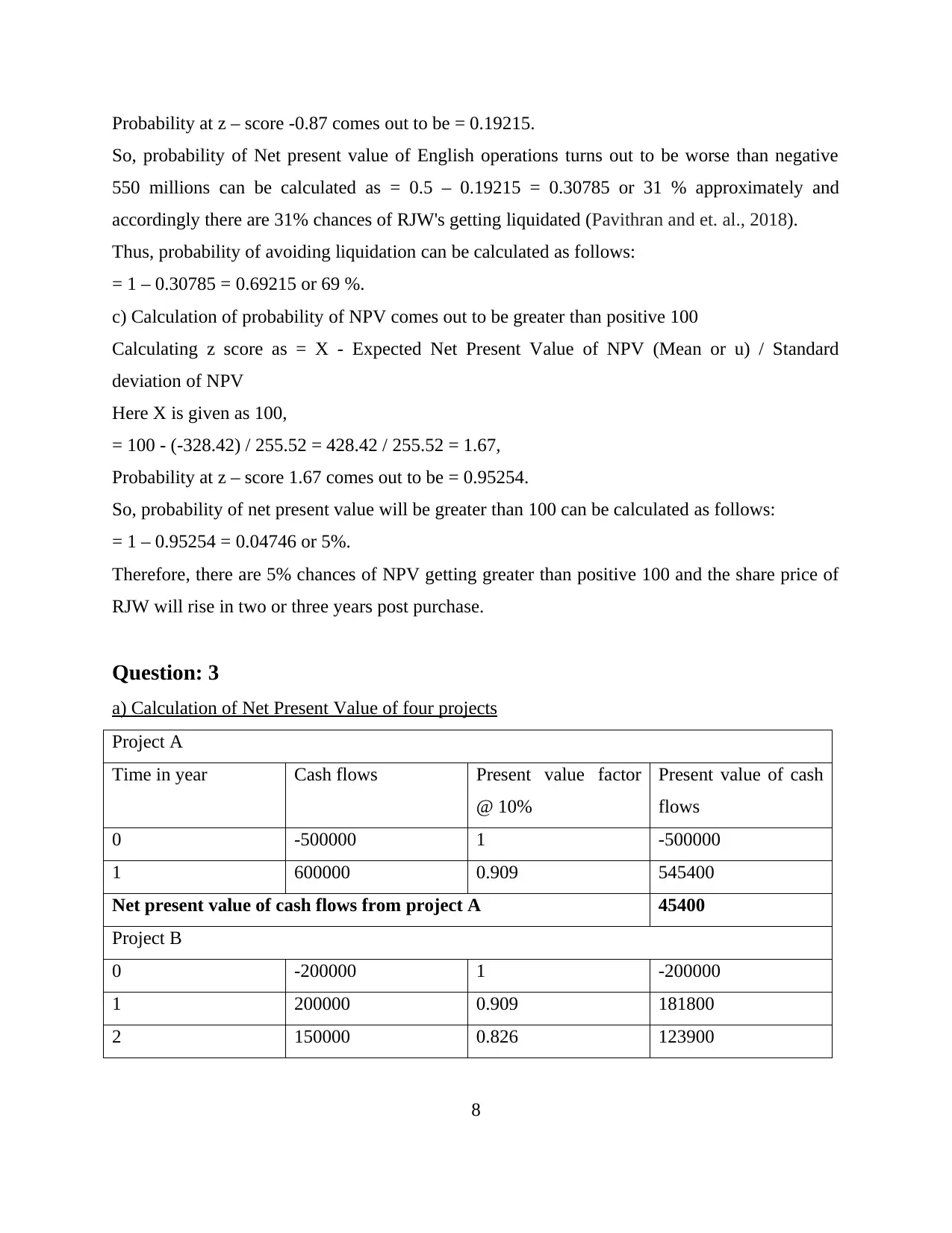
Probability at z – score -0.87 comes out to be = 0.19215.
So, probability of Net present value of English operations turns out to be worse than negative
550 millions can be calculated as = 0.5 – 0.19215 = 0.30785 or 31 % approximately and
accordingly there are 31% chances of RJW's getting liquidated (Pavithran and et. al., 2018).
Thus, probability of avoiding liquidation can be calculated as follows:
= 1 – 0.30785 = 0.69215 or 69 %.
c) Calculation of probability of NPV comes out to be greater than positive 100
Calculating z score as = X - Expected Net Present Value of NPV (Mean or u) / Standard
deviation of NPV
Here X is given as 100,
= 100 - (-328.42) / 255.52 = 428.42 / 255.52 = 1.67,
Probability at z – score 1.67 comes out to be = 0.95254.
So, probability of net present value will be greater than 100 can be calculated as follows:
= 1 – 0.95254 = 0.04746 or 5%.
Therefore, there are 5% chances of NPV getting greater than positive 100 and the share price of
RJW will rise in two or three years post purchase.
Question: 3
a) Calculation of Net Present Value of four projects
Project A
Time in year Cash flows Present value factor
@ 10%
Present value of cash
flows
0 -500000 1 -500000
1 600000 0.909 545400
Net present value of cash flows from project A 45400
Project B
0 -200000 1 -200000
1 200000 0.909 181800
2 150000 0.826 123900
8

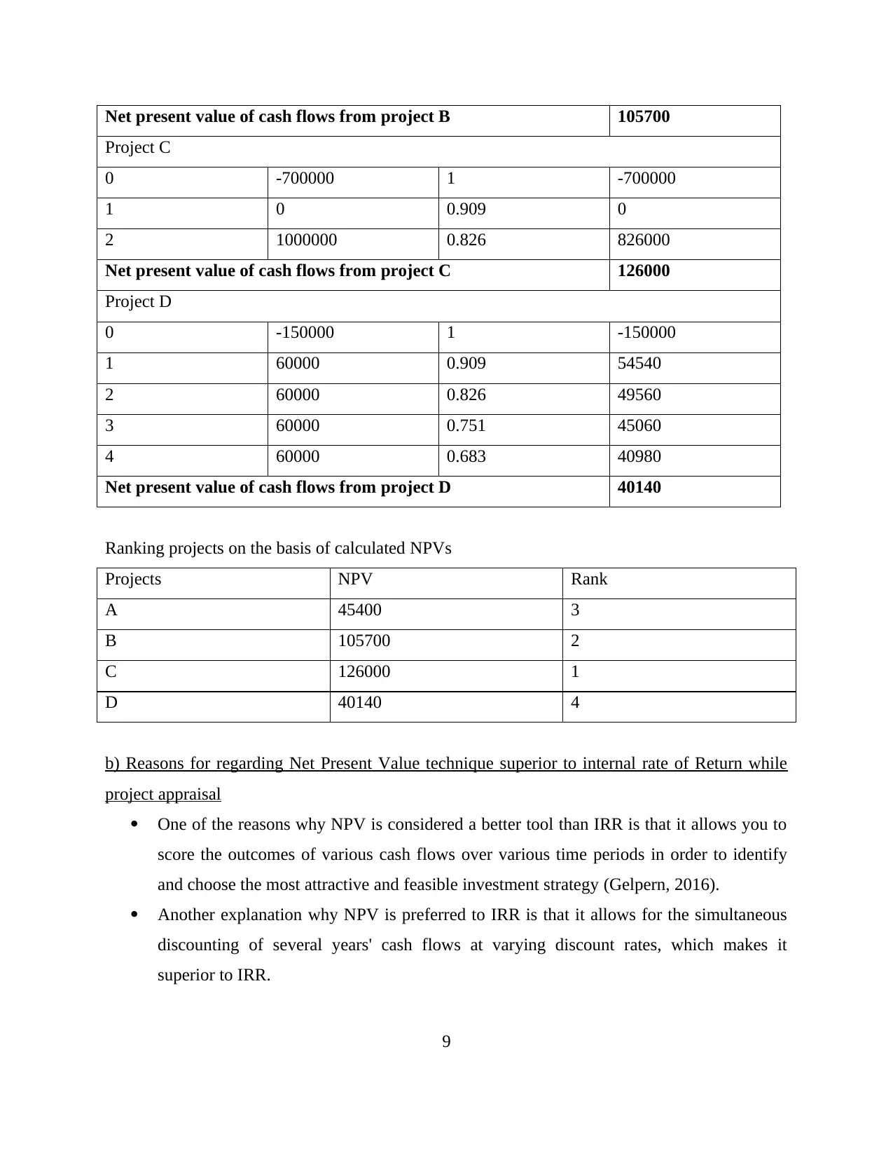
Net present value of cash flows from project B 105700
Project C
0 -700000 1 -700000
1 0 0.909 0
2 1000000 0.826 826000
Net present value of cash flows from project C 126000
Project D
0 -150000 1 -150000
1 60000 0.909 54540
2 60000 0.826 49560
3 60000 0.751 45060
4 60000 0.683 40980
Net present value of cash flows from project D 40140
Ranking projects on the basis of calculated NPVs
Projects NPV Rank
A 45400 3
B 105700 2
C 126000 1
D 40140 4
b) Reasons for regarding Net Present Value technique superior to internal rate of Return while
project appraisal
 One of the reasons why NPV is considered a better tool than IRR is that it allows you to
score the outcomes of various cash flows over various time periods in order to identify
and choose the most attractive and feasible investment strategy (Gelpern, 2016).
 Another explanation why NPV is preferred to IRR is that it allows for the simultaneous
discounting of several years' cash flows at varying discount rates, which makes it
superior to IRR.
9

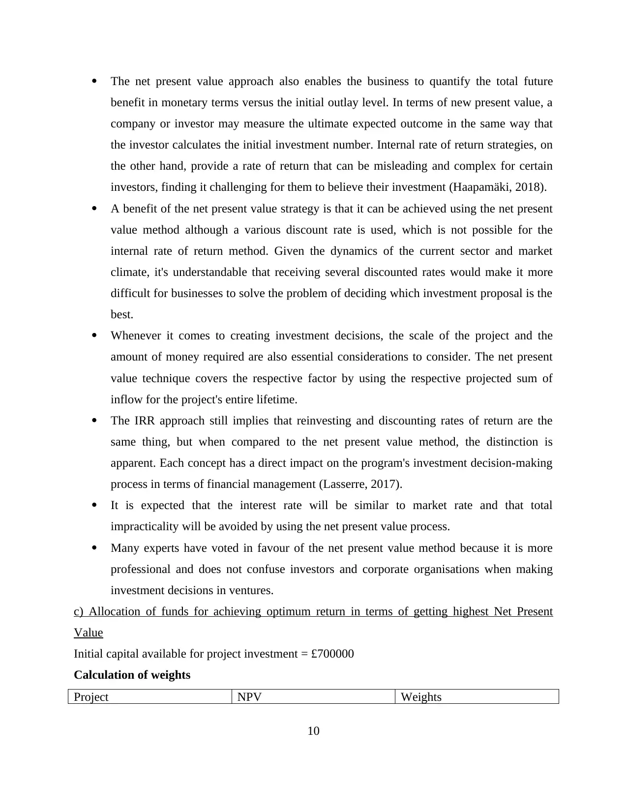
 The net present value approach also enables the business to quantify the total future
benefit in monetary terms versus the initial outlay level. In terms of new present value, a
company or investor may measure the ultimate expected outcome in the same way that
the investor calculates the initial investment number. Internal rate of return strategies, on
the other hand, provide a rate of return that can be misleading and complex for certain
investors, finding it challenging for them to believe their investment (Haapamäki, 2018).
 A benefit of the net present value strategy is that it can be achieved using the net present
value method although a various discount rate is used, which is not possible for the
internal rate of return method. Given the dynamics of the current sector and market
climate, it's understandable that receiving several discounted rates would make it more
difficult for businesses to solve the problem of deciding which investment proposal is the
best.
 Whenever it comes to creating investment decisions, the scale of the project and the
amount of money required are also essential considerations to consider. The net present
value technique covers the respective factor by using the respective projected sum of
inflow for the project's entire lifetime.
 The IRR approach still implies that reinvesting and discounting rates of return are the
same thing, but when compared to the net present value method, the distinction is
apparent. Each concept has a direct impact on the program's investment decision-making
process in terms of financial management (Lasserre, 2017).
 It is expected that the interest rate will be similar to market rate and that total
impracticality will be avoided by using the net present value process.
 Many experts have voted in favour of the net present value method because it is more
professional and does not confuse investors and corporate organisations when making
investment decisions in ventures.
c) Allocation of funds for achieving optimum return in terms of getting highest Net Present
Value
Initial capital available for project investment = £700000
Calculation of weights
Project NPV Weights
10

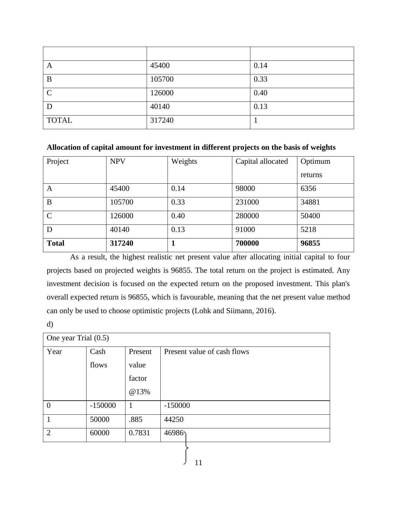
A 45400 0.14
B 105700 0.33
C 126000 0.40
D 40140 0.13
TOTAL 317240 1
Allocation of capital amount for investment in different projects on the basis of weights
Project NPV Weights Capital allocated Optimum
returns
A 45400 0.14 98000 6356
B 105700 0.33 231000 34881
C 126000 0.40 280000 50400
D 40140 0.13 91000 5218
Total 317240 1 700000 96855
As a result, the highest realistic net present value after allocating initial capital to four
projects based on projected weights is 96855. The total return on the project is estimated. Any
investment decision is focused on the expected return on the proposed investment. This plan's
overall expected return is 96855, which is favourable, meaning that the net present value method
can only be used to choose optimistic projects (Lohk and Siimann, 2016).
d)
One year Trial (0.5)
Year Cash
flows
Present
value
factor
@13%
Present value of cash flows
0 -150000 1 -150000
1 50000 .885 44250
2 60000 0.7831 46986
11

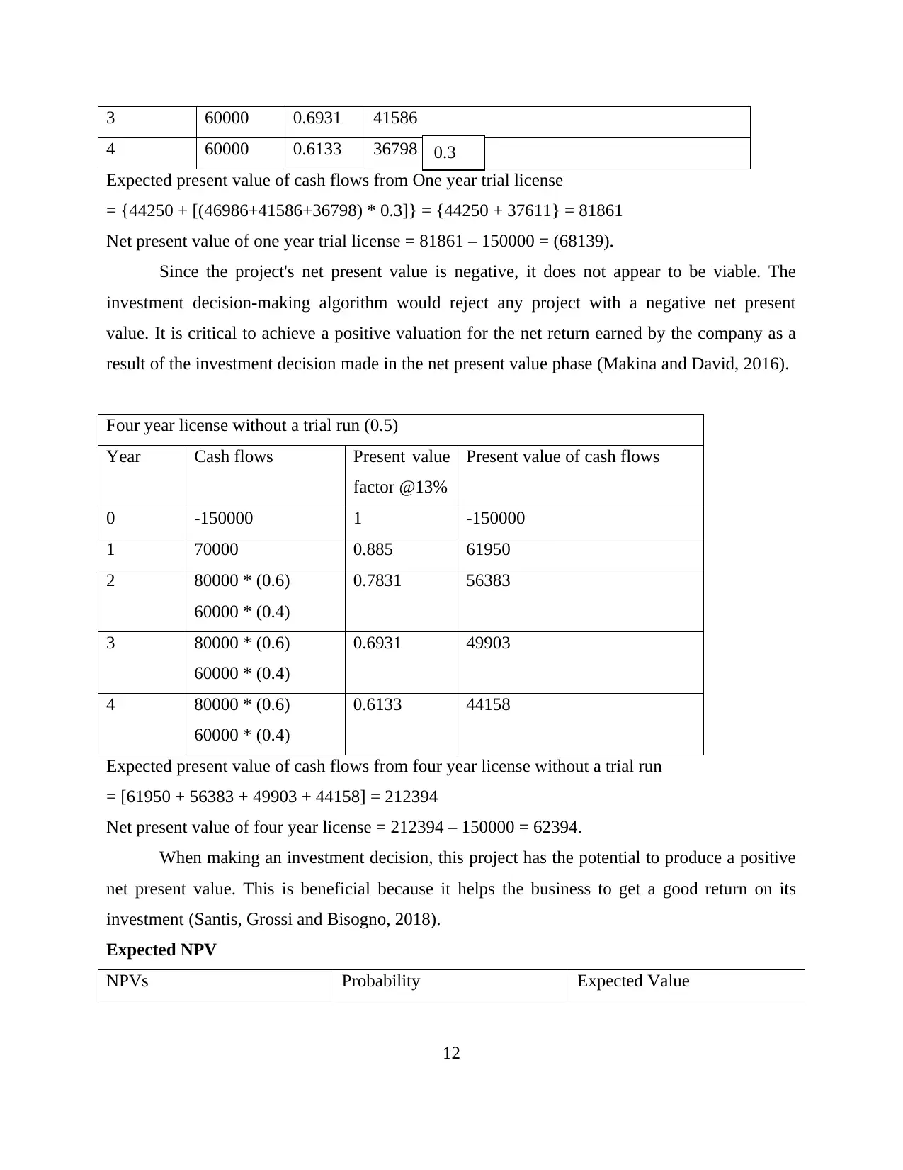
3 60000 0.6931 41586
4 60000 0.6133 36798
Expected present value of cash flows from One year trial license
= {44250 + [(46986+41586+36798) * 0.3]} = {44250 + 37611} = 81861
Net present value of one year trial license = 81861 – 150000 = (68139).
Since the project's net present value is negative, it does not appear to be viable. The
investment decision-making algorithm would reject any project with a negative net present
value. It is critical to achieve a positive valuation for the net return earned by the company as a
result of the investment decision made in the net present value phase (Makina and David, 2016).
Four year license without a trial run (0.5)
Year Cash flows Present value
factor @13%
Present value of cash flows
0 -150000 1 -150000
1 70000 0.885 61950
2 80000 * (0.6)
60000 * (0.4)
0.7831 56383
3 80000 * (0.6)
60000 * (0.4)
0.6931 49903
4 80000 * (0.6)
60000 * (0.4)
0.6133 44158
Expected present value of cash flows from four year license without a trial run
= [61950 + 56383 + 49903 + 44158] = 212394
Net present value of four year license = 212394 – 150000 = 62394.
When making an investment decision, this project has the potential to produce a positive
net present value. This is beneficial because it helps the business to get a good return on its
investment (Santis, Grossi and Bisogno, 2018).
Expected NPV
NPVs Probability Expected Value
12
0.3

(68139) 0.5 -34070
62394 0.5 31197
Expected NPV -2873
Standard deviation of NPV
Events NPVs D = (NPV –
Expected
NPV)
D2 P =
Probability
PD2
One year trial (68139) -65266 4,259,650,756 0.5 2,129,825,378
Four year
license
62394 65231 4,255,083,361 0.5 2,127,541,680
Variance 4257367058
Standard deviation 65248
Calculation of z-score, where it is know that all the values below 0 will results in negative NPV.
So, here X is equals to 0.
Z – Score = 0 – expected NPV / standard deviation of NPV = 0 – (-2873) / 65248 = 2873 / 65248
= 0.044.
Probability of negative NPV from 0 till Expected NPV = 0.017548 or 1.7548 %.
Therefore, Probability of negative NPV = 0.5 + 0.017548 = 0.5175 or 51.75%.
A negative net present value factor is included in any strategy, indicating that the
business entity's investment decision must be balanced against the possibility of a negative
present value. Negative also means that the business would not see a return on its project
expenditure (Saksonova and Savina, 2016). This will make profiting from the investment
proposal selected by the corporation even more complicated for the business organisation. The
key advantage of the net present value approach is that it gives the entity precise information
about the project's overall possible benefits.
13

CONCLUSION
Investment decision-making involves evaluating the state of a business entity and making
the best possible decision that will result in the best possible financial results for the business
entity. The return obtained from the investment plan in front of the company is the primary basis
for making investment decisions. The net present value approach is a vital business decision-
making technique that assists a company in determining the best investment decision for a
project. This technique is all about the difference between the return provided by a decision and
the initial amount of investment made in a project. All of this allows the entity to make the best
possible decision.
14

REFERENCES
Books and journals
Belasri, S., Gomes, M. and Pijourlet, G., 2020. Corporate social responsibility and bank
efficiency. Journal of Multinational Financial Management, 54, p.100612.
De Smet, D., Mention, A.L. and Torkkeli, M., 2016. Involving high net worth individuals
(HNWI) for financial services innovation. Journal of Financial Services Marketing,
21(3), pp.226-239.
Duque-Grisales, E. and Aguilera-Caracuel, J., 2019. Environmental, social and governance
(ESG) scores and financial performance of Multilatinas: Moderating effects of
geographic international diversification and financial slack. Journal of Business Ethics,
pp.1-20.
Enomoto, M., Kimura, F. and Yamaguchi, T., 2018. A cross‐country study on the relationship
between financial development and earnings management. Journal of International
Financial Management & Accounting, 29(2), pp.166-194.
Ferris, S.P., Javakhadze, D. and Rajkovic, T., 2019. An international analysis of CEO social
capital and corporate risk‐taking. European Financial Management, 25(1), pp.3-37.
Gelpern, A., 2016. Financial services. Trans-Pacific Partnership: An Assessment, 104, p.171.
Haapamäki, E., 2018. How has IFRS impacted financial reporting for unlisted entities?. Journal
of Accounting and Management Information Systems, 17(1), pp.5-30.
Lasserre, P., 2017. Global strategic management. Macmillan International Higher Education.
Lohk, P. and Siimann, P., 2016, December. Predicting the risk of encountering financial
difficulties by the example of Estonian municipalities. In 5th International Conference
on Accounting, Auditing, and Taxation (ICAAT 2016) (pp. 297-306). Atlantis Press.
Makina, C. and David, M., 2016. Public Financial Accountability: A pre-requisite to the
management of Development Assistance in Mozambique beyond 2015. Africa’s Public
Service Delivery and Performance Review, 4(4), pp.554-572.
Saksonova, S. and Savina, S., 2016. Financial Management as a Tool for Achieving Stable Firm
Growth. Economics & Business, 29(1).
Santis, S., Grossi, G. and Bisogno, M., 2018. Public sector consolidated financial statements: a
structured literature review. Journal of Public Budgeting, Accounting & Financial
Management.
15