401077 Biostatistics Assignment 1: Data Analysis from Framingham Study

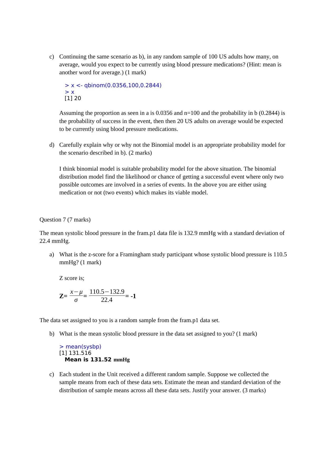
This biostatistics assignment, focusing on the Framingham Study, requires students to analyze a dataset using R Commander. The assignment begins by exploring quantitative variables and the rationale behind them, along with identifying variables. Students are tasked with graphing distributions of serum total cholesterol and attained education, providing descriptive summaries of each. Relationships between variables, such as serum cholesterol and attained education, are examined through graphs and statistical analysis. Furthermore, the assignment explores the relationship between gender and cigarette smoking using tables and probability calculations, including conditional probabilities. The binomial probability model is applied to estimate probabilities related to blood pressure medication use. The assignment concludes with z-score calculations for systolic blood pressure and estimation of the mean and standard deviation of sample means, along with the proportion of samples with a sample mean smaller than a reported value.

401077 Introduction to Biostatistics, Autumn 2020
Assignment 1 (Due Sunday March 29, 2020)
Please answer all 7 questions. Record your answers in the template document provided and submit via
Turnitin before 11:59pm on the due date. The marks allocated to each question are shown in the
assignment. A total of 30 marks are available and this assignment is worth 30% of your overall grade.
Some of the questions require you to analyse the unique assignment data set which I have created for
you. This is labelled ‘dataforxxxxxxxx.RData’ where xxxxxxxx represents your Student ID number.
The description of this data set is provided in the file ‘Description of your data set.docx’. You can
find your data set and its description into the Assessment 1 folder in vUWS.
Note: Each student will get different answers as the data sets differ.
Question 1 (2 marks)
Consider the sample from the Framingham Study assigned to you for your assignment.
a) Explain why heart rate (heartrte) is a quantitative variable. (1 mark)
Quantitative variables are variables with numerical values where arithmetic operations such
as addition, multiplication, subtraction and division can be carried on. The heart rate is
numeric and these operation can suffice. For instance it is possible to compute the mean heart
rate for the data hence it is quantitative.
b) Explain why your student number (yourID) is not a variable. (1 mark)
The student number is only important in tracing the questionnaires and where the data
originated from. It cannot be useful in making any generalization on the data hence it is not a
variable.
Question 2 (4 marks)
a) Using the sample from the Framingham Study assigned to you and R Commander, graph the
distribution of serum total cholesterol (totchol). Provide an appropriate title and descriptive
axis labels. (1 mark)
Histogram can be used to show the distribution serum total cholesterol (totchol) as follows;

b) Using appropriate statistics from R Commander, write one or two sentences describing the
distribution of serum total cholesterol (totchol). (Hint: consider measures of centre, spread
and shape. R commander output alone is insufficient – write the answer in your own words.)
(3 marks)
Min. 1st Qu. Median Mean 3rd Qu. Max. NA's
133 205 232 234 256 600 4
As seen in the histogram above,the total cholesterol distribution is positively skewed.More
data if found on the right hand side.The value of mean >median hence shoving that the data is right-
skewed.The mean cholesterol for all the subjects was 234 mg/dL with a median of 232 mg/dL.The
standard deviation was 43.50 mg/dL.The lowest recorded cholesterol amount was 133 mg/dL with
600 mg/dL being the highest amount of cholesterol recorded.
Question 3 (3 marks)
Using the sample from the Framingham Study assigned to you and R Commander, graph the
frequency distribution of ‘Attained education’ (educ_f). Provide an appropriate title and descriptive
axis labels. Write a sentence or two summarising the main characteristics of this distribution as shown
by the graph. (3 marks)
The Attained education was "0-11 years", "High school diploma", "Some college", “College degree"
with frequency distribution of 132, 86, 46 and 39 respectively. These were substituted with letters to
fit in the bar graph such as 0-11 years-A, High school diploma-B, Some college-C, and College
degree-D
The results revealed a skewed distribution where the distribution of subjects decreased with increase
with education level. The study subjects who had attained less education were more compared to them
that had attained higher education.

Question 4 (4 marks)
Using the sample from the Framingham Study assigned to you and R Commander, graph respondents’
‘serum total cholesterol’ (totchol) against ‘Attained education’ (educ_f). ). Provide an appropriate title
and descriptive axis labels. Using the graph and associated statistics, write a sentence or two
describing the relationship between these two variables. (4 marks)

The Attained education was "0-11 years", "High school diploma", "Some college", “College degree"
were represented by 1.0,2.0,3.0 and 4.0 respectively in the above graph. It can be noted that High
school had the student with the highest cholesterol amount totalling to 600which is probably an
outlier. The population seems to have less cholesterol as they attain higher education.
Question 5 (5 marks)
a) Using the sample from the Framingham Study assigned to you and R Commander, tabulate
the relationship between gender (sex) and current cigarette smoking (cursmok). Include
frequency counts and either row or column percentages. (Hint: R commander output alone is
insufficient – present your table(s) in Word with informative headings.) (1 mark)
cursmoke
sex Not current smoker Current smoker
male 52 61
female 115 85
Column
Percentages
sex
cursmoke
Not currrent
smoker Currrent smoker Total
male 31% 42% 73%
female 69% 58% 127%
Total 100% 100% 200
sex
cursmoke
Not currrent
smoker Currrent smoker Total
male 52 61 113
female 115 85 200
Total 167 146 313

b) Using the results in part a) write a sentence or two describing the relationship between gender
and current cigarette smoking. (2 mark)
Out of the sampled subjects ,the higher percentage of current smokers were found to be
females(58%) compared to males(42%)
c) If you were to select one person at random from this data set, what is the probability they
would be a male and a current cigarette smoker? (1 mark)
P(Male) and P(Current smoker)=P(113/313)*(146/313)=0.361*0.466=0.1684
d) If you were to choose one female at random from this data set, what is the probability they
would be a current cigarette smoker? (1 mark)
P(Female) and P(Current smoker)=P(200/313)*(146/313)=0.639*0.466=0.298
Question 6 (5 marks)
a) Using the sample from the Framingham Study assigned to you, what proportion of people in
your data set are coded as currently using blood pressure medications (bpmeds=Current use)?
(1 mark)
bpmeds
Not currently used Currently used
298 11
Total=298+11=309
Proportion (bpmeds=Current use)=11/309=0.0356
b) Suppose your answer in a) was the proportion of adults in the US currently using blood
pressure medication. Suppose you take a random sample of size 100 from all US adults and
ask them if they were currently using blood pressure medication. Use the Binomial
probability model and R Commander to estimate the probability that more than 5 of these 100
would be currently using blood pressure medication. (Hint: To avoid any problems in R
Commander, use a number slightly more than 5 such as 5.1.) (1 mark)
X∼Bin(n,p) implying that X~Bin(100, 0.0356)
c<-pbinom(4, size=100, prob=0.0356)
> c
[1] 0.7156247
> 1-c
[1] 0.2843753
P(X>5) for Bin(100, 0.0356)=0.2844

c) Continuing the same scenario as b), in any random sample of 100 US adults how many, on
average, would you expect to be currently using blood pressure medications? (Hint: mean is
another word for average.) (1 mark)
> x <- qbinom(0.0356,100,0.2844)
> x
[1] 20
Assuming the proportion as seen in a is 0.0356 and n=100 and the probability in b (0.2844) is
the probability of success in the event, then then 20 US adults on average would be expected
to be currently using blood pressure medications.
d) Carefully explain why or why not the Binomial model is an appropriate probability model for
the scenario described in b). (2 marks)
I think binomial model is suitable probability model for the above situation. The binomial
distribution model find the likelihood or chance of getting a successful event where only two
possible outcomes are involved in a series of events. In the above you are either using
medication or not (two events) which makes its viable model.
Question 7 (7 marks)
The mean systolic blood pressure in the fram.p1 data file is 132.9 mmHg with a standard deviation of
22.4 mmHg.
a) What is the z-score for a Framingham study participant whose systolic blood pressure is 110.5
mmHg? (1 mark)
Z score is;
Z= x−μ
σ = 110.5−132.9
22.4 = -1
The data set assigned to you is a random sample from the fram.p1 data set.
b) What is the mean systolic blood pressure in the data set assigned to you? (1 mark)
> mean(sysbp)
[1] 131.516
Mean is 131.52 mmHg
c) Each student in the Unit received a different random sample. Suppose we collected the
sample means from each of these data sets. Estimate the mean and standard deviation of the
distribution of sample means across all these data sets. Justify your answer. (3 marks)

One approach is to compute the grand mean. This is the general means of the sample
means and also the sample standard deviation of all the samples generated. This will
determine the estimate of the population mean and standard deviation.
d) Calculate the z-score for the sample mean you reported in b). (1 mark)
Z= x−μ
σ = 131.52−132.9
22.4 = -0.06161
e) Using R Commander, estimate the proportion of samples which would have a sample mean
smaller than the sample mean you reported in b). (1 mark)
> mean(sysbp<132.52)
[1] 0.5878594
=184/313=0.5878 i.e 58.79%

References
Gupta, S. C., & Kapoor, V. K (2019) Fundamentals of applied statistics. Sulthan Chand &
Sons,
King'oriah, G. K.(2012) "Fundamentals of applied statistics." Nairobi: The Jomo Kenyatta
Foundation.
Lee, A. J. U-statistics: (2019)Theory and Practice. Routledge
Sullivan, M., & Verhoosel, J. C. M.( 2013).Statistics: Informed decisions using data. New
York, NY: Pearson.