Inventory Control System Analysis: Case Study and Solutions

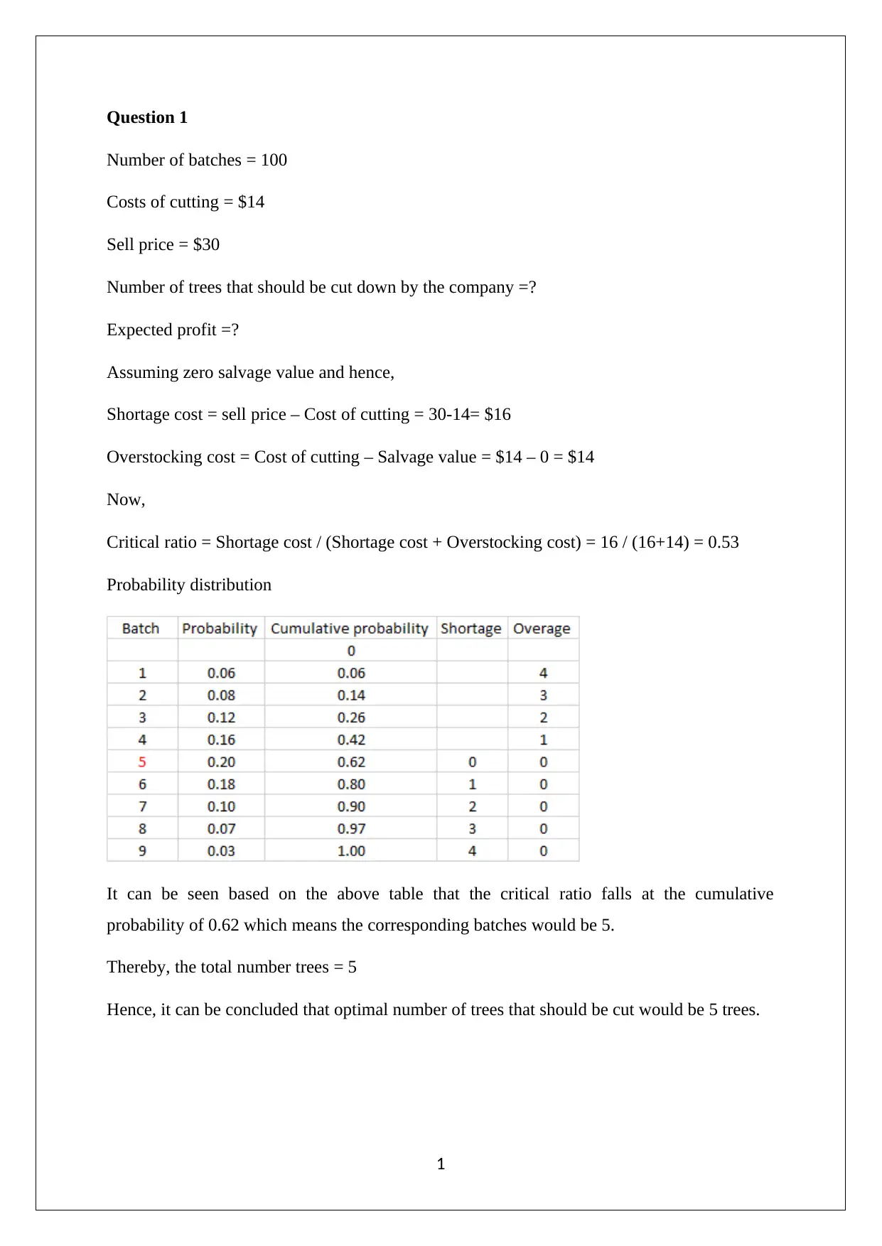
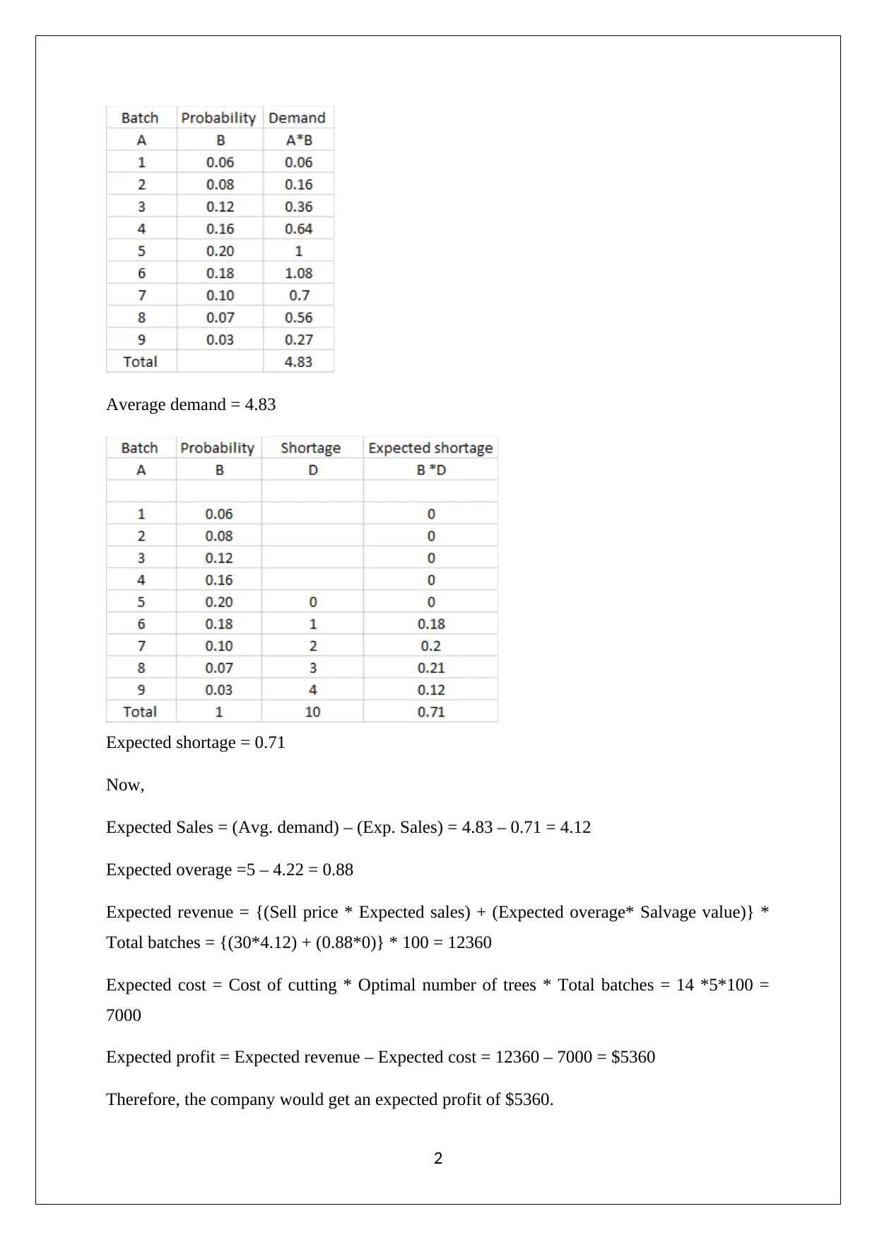
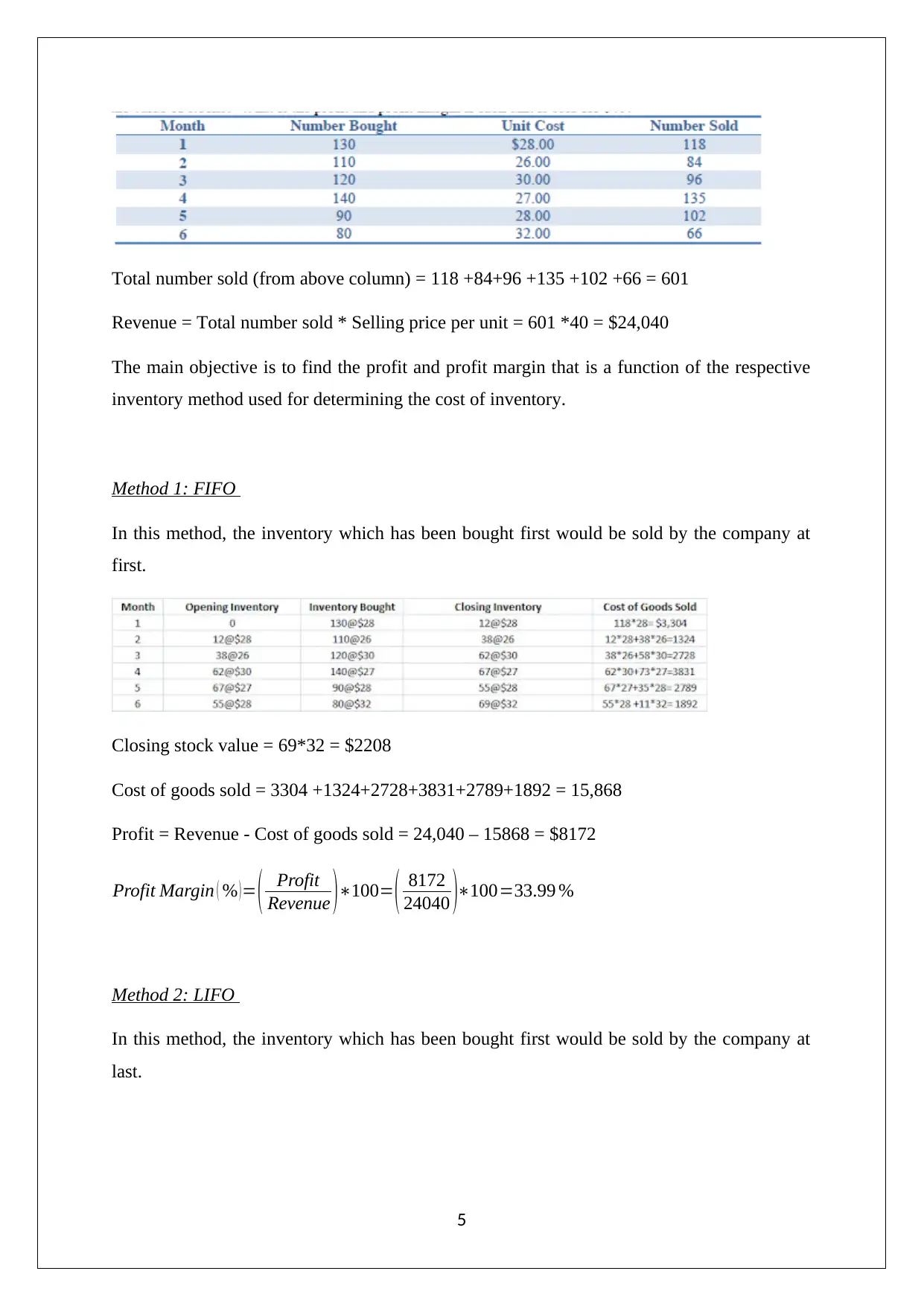
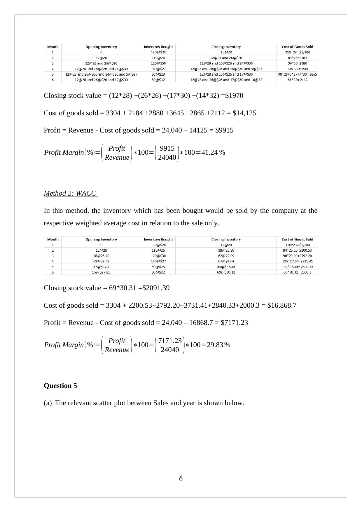
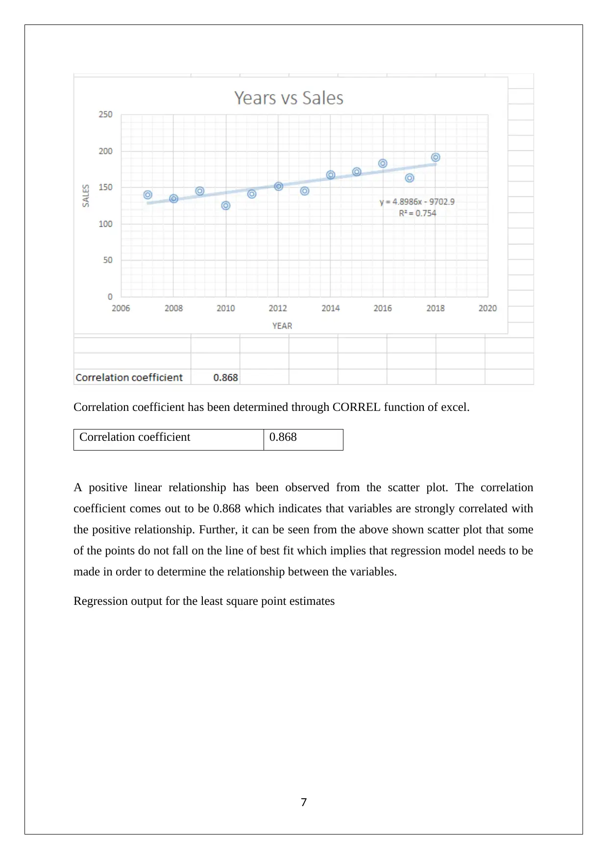
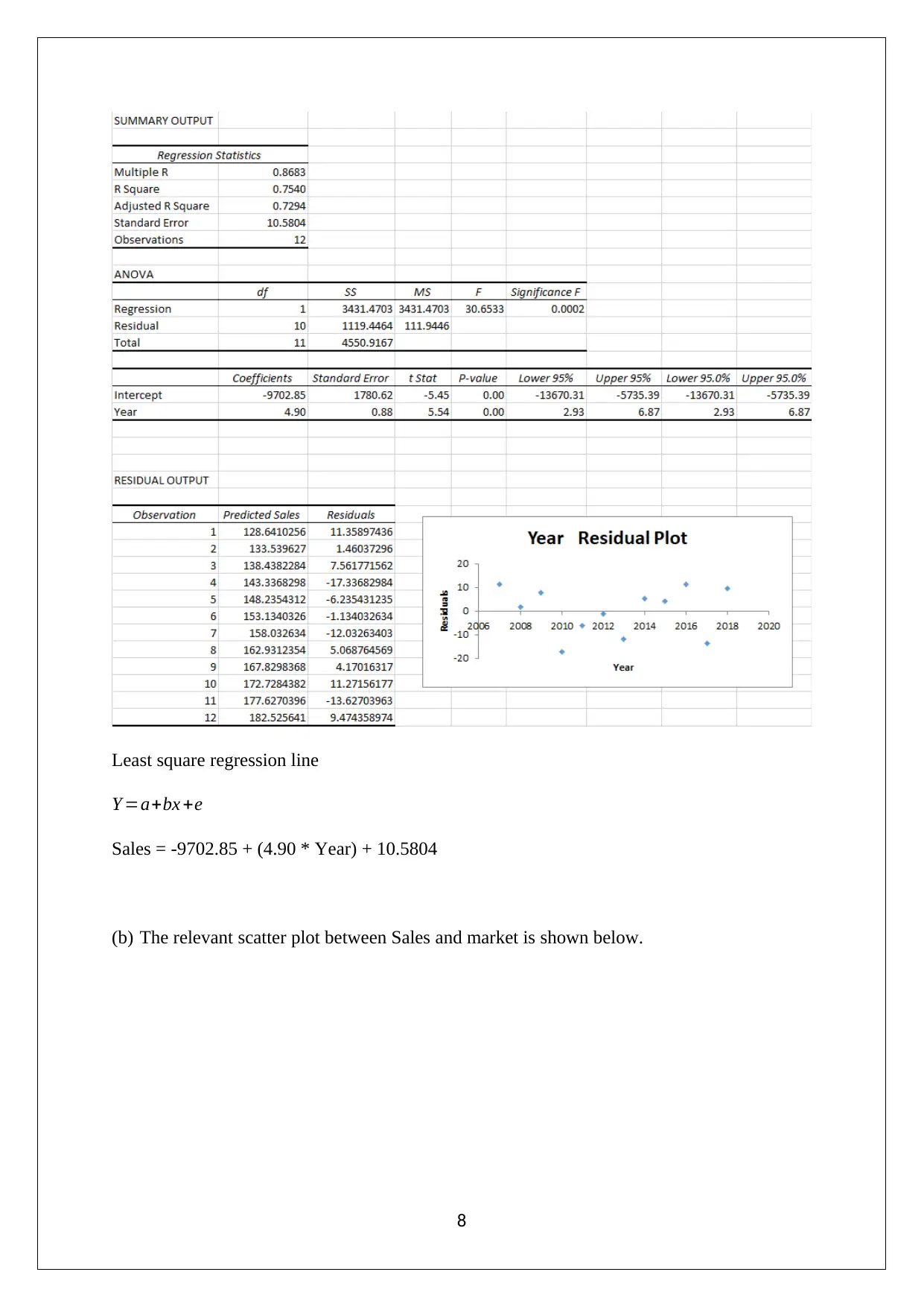
This document presents a comprehensive solution to an inventory control assignment, addressing various aspects of inventory management. The solution begins with an analysis of optimal tree cutting quantities, considering shortage and overstocking costs to determine the expected profit. It then delves into Economic Order Quantity (EOQ) calculations, followed by a detailed examination of reorder points (ROP) and safety stock, including adjustments for different service levels. The assignment further explores inventory costing methods, comparing the impact of FIFO, LIFO, and Weighted Average Cost (WACC) on profit margins. Finally, it incorporates regression analysis to forecast sales based on year and market data, identifying the most appropriate model for sales prediction. This assignment provides a practical application of inventory management techniques and statistical analysis within a business context.

Inventory control system
[Document subtitle]
[DATE]

Question 1
Number of batches = 100
Costs of cutting = $14
Sell price = $30
Number of trees that should be cut down by the company =?
Expected profit =?
Assuming zero salvage value and hence,
Shortage cost = sell price – Cost of cutting = 30-14= $16
Overstocking cost = Cost of cutting – Salvage value = $14 – 0 = $14
Now,
Critical ratio = Shortage cost / (Shortage cost + Overstocking cost) = 16 / (16+14) = 0.53
Probability distribution
It can be seen based on the above table that the critical ratio falls at the cumulative
probability of 0.62 which means the corresponding batches would be 5.
Thereby, the total number trees = 5
Hence, it can be concluded that optimal number of trees that should be cut would be 5 trees.
1

Average demand = 4.83
Expected shortage = 0.71
Now,
Expected Sales = (Avg. demand) – (Exp. Sales) = 4.83 – 0.71 = 4.12
Expected overage =5 – 4.22 = 0.88
Expected revenue = {(Sell price * Expected sales) + (Expected overage* Salvage value)} *
Total batches = {(30*4.12) + (0.88*0)} * 100 = 12360
Expected cost = Cost of cutting * Optimal number of trees * Total batches = 14 *5*100 =
7000
Expected profit = Expected revenue – Expected cost = 12360 – 7000 = $5360
Therefore, the company would get an expected profit of $5360.
2

Question 2
D = 12.5
R = $65
S = $170
H = $7
L= 1
Optimal Value of Order Quantity ¿ ( 2∗D∗S
H )
0.5
Optimal Value of Order Quantity=( 2∗12.5∗170
7 )0.5
=24.64∨25
Reorder Level = DL = 12.5 * 1 = 12.5
Question 3
Service level = 95%
Mean demand of the company = 280 units a week
Standard deviation = 38 units
lead time = 2.2 weeks (Constant)
Company’s practice for this item would constitute the ROP and safety stock.
Safety Stock
Safety stock=Z∗standard deviation∗( Lead time ) 0.5
z value for 95 %service level=1.65
Safety stock=1.65∗38∗( 2.2 ) 0.5=92.9∨93
ROP
3

ROP=(Mean∗Lead time)+¿
ROP= ( 280∗2.2 ) + ( 1.65∗38∗( 2.2 ) 0.5 ) =708.9∨709
Company’s practice for this item would constitute 709 ROP and 93 safety stock.
Now, the annual cost associated with this scenario is shown below.
= {(100*280)+(709-280)*400 }/52 = $3838.46
Company’s practice for this item would constitute the ROP and safety stock when service
level is 98%.
Safety Stock
Safety stock=Z∗standard deviation∗( Lead time ) 0.5
z value for 98 %service level=2.055
Safety stock=2.055∗38∗( 2.2 ) 0.5 =115.8∨116
ROP
ROP=(Mean∗Lead time)+¿
ROP= ( 280∗2.2 ) + ( 1.65∗38∗( 2.2 ) 0.5 ) =731.82∨732
Company’s practice for this item would constitute 732 ROP and 116 safety stock when the
service level has increased to 98% from 95%.
Question 4
Given data and information is shown below.
Selling price per unit = $40
4

Total number sold (from above column) = 118 +84+96 +135 +102 +66 = 601
Revenue = Total number sold * Selling price per unit = 601 *40 = $24,040
The main objective is to find the profit and profit margin that is a function of the respective
inventory method used for determining the cost of inventory.
Method 1: FIFO
In this method, the inventory which has been bought first would be sold by the company at
first.
Closing stock value = 69*32 = $2208
Cost of goods sold = 3304 +1324+2728+3831+2789+1892 = 15,868
Profit = Revenue - Cost of goods sold = 24,040 – 15868 = $8172
Profit Margin ( % )= ( Profit
Revenue )∗100= ( 8172
24040 )∗100=33.99 %
Method 2: LIFO
In this method, the inventory which has been bought first would be sold by the company at
last.
5

Closing stock value = (12*28) +(26*26) +(17*30) +(14*32) =$1970
Cost of goods sold = 3304 + 2184 +2880 +3645+ 2865 +2112 = $14,125
Profit = Revenue - Cost of goods sold = 24,040 – 14125 = $9915
Profit Margin ( % )= ( Profit
Revenue )∗100= ( 9915
24040 )∗100=41.24 %
Method 2: WACC
In this method, the inventory which has been bought would be sold by the company at the
respective weighted average cost in relation to the sale only.
Closing stock value = 69*30.31 =$2091.39
Cost of goods sold = 3304 + 2200.53+2792.20+3731.41+2840.33+2000.3 = $16,868.7
Profit = Revenue - Cost of goods sold = 24,040 – 16868.7 = $7171.23
Profit Margin ( % ) = ( Profit
Revenue )∗100= ( 7171.23
24040 )∗100=29.83 %
Question 5
(a) The relevant scatter plot between Sales and year is shown below.
6

Correlation coefficient has been determined through CORREL function of excel.
Correlation coefficient 0.868
A positive linear relationship has been observed from the scatter plot. The correlation
coefficient comes out to be 0.868 which indicates that variables are strongly correlated with
the positive relationship. Further, it can be seen from the above shown scatter plot that some
of the points do not fall on the line of best fit which implies that regression model needs to be
made in order to determine the relationship between the variables.
Regression output for the least square point estimates
7

Least square regression line
Y =a+bx +e
Sales = -9702.85 + (4.90 * Year) + 10.5804
(b) The relevant scatter plot between Sales and market is shown below.
8

Correlation coefficient has been determined through CORREL
function of excel.
Correlation coefficient 0.661
A positive linear relationship has been observed from the scatter plot between the variables.
The correlation coefficient comes out to be 0.661 which indicates that variables are positively
moderately correlated. Further, it can be seen from the above shown scatter plot that some of
the points do not fall on the line of best fit which implies that regression model needs to be
made in order to determine the relationship between the variables.
Regression output for the least square point estimates
9

Least square regression line
Y =a+bx +e
Sales = 53.44 + (0.91 * Market) + 16.016
(c) The most appropriate model would be the first one where the dependent variable is sales
and independent variable is year. This is because the R square value comes out to be
higher for model one. Also, the sales seem to follows a linearity with respect to the year
and thus, the sales would be best explained through year rather than market and thus, it
would be preferable model.
10

11