Comprehensive Inventory Control System Assignment with Solutions

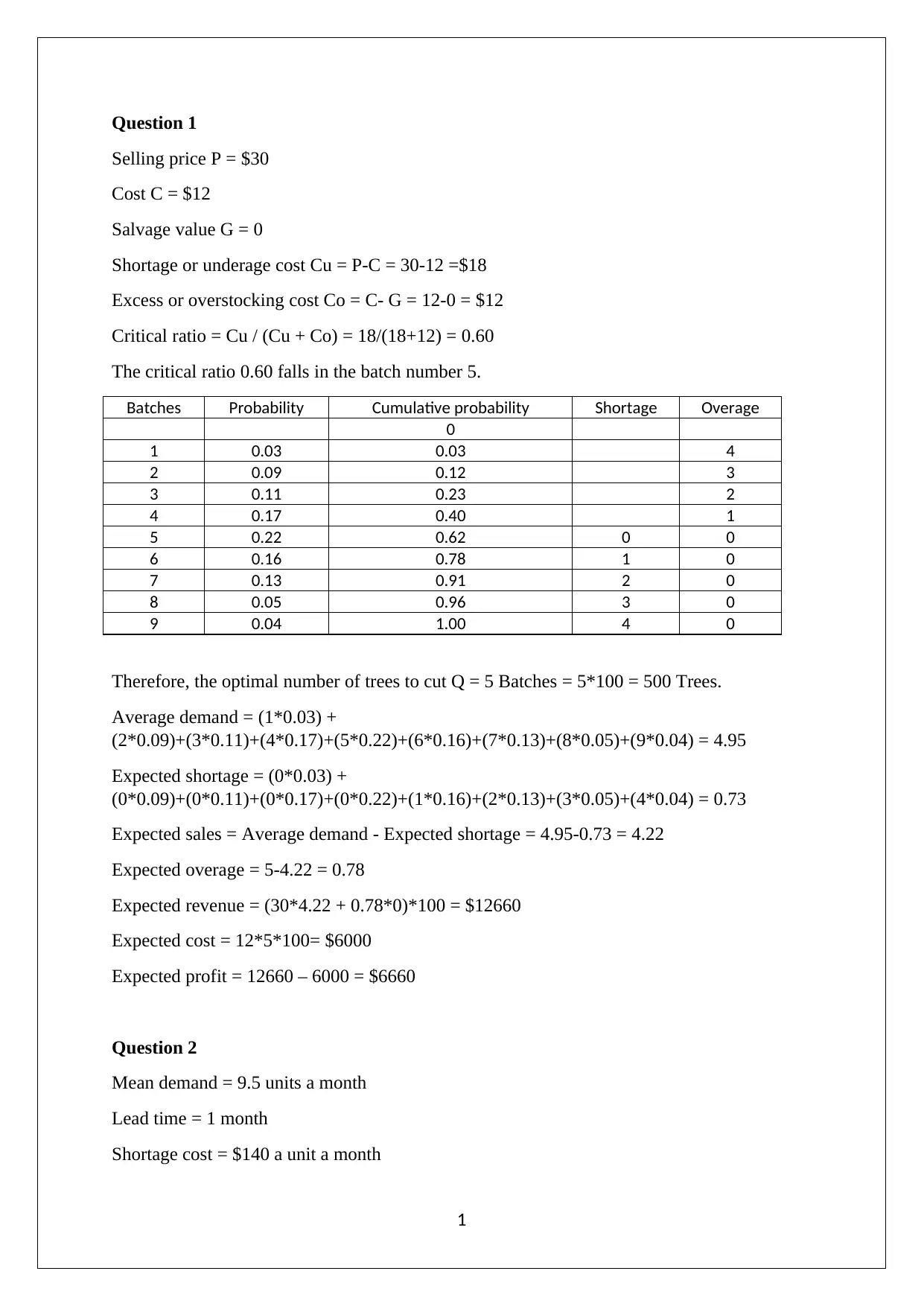
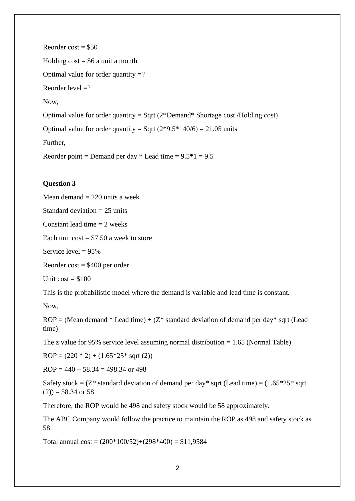
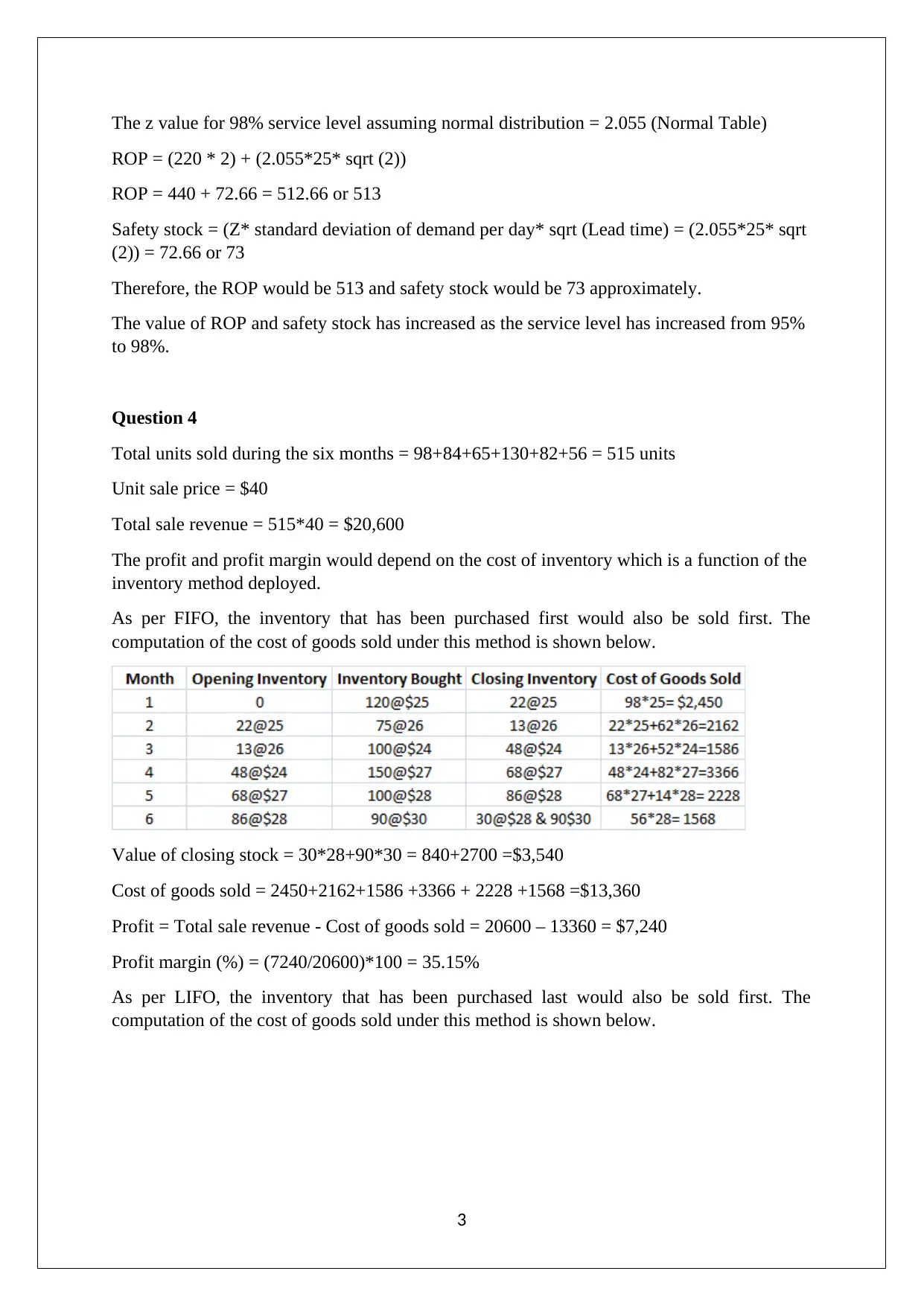
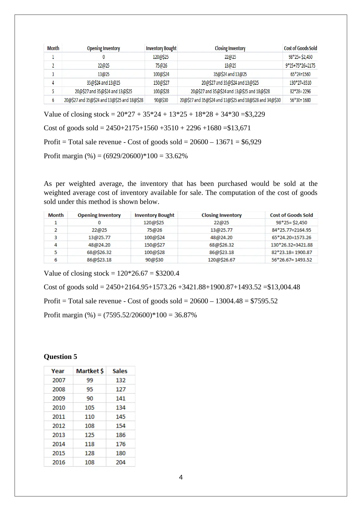
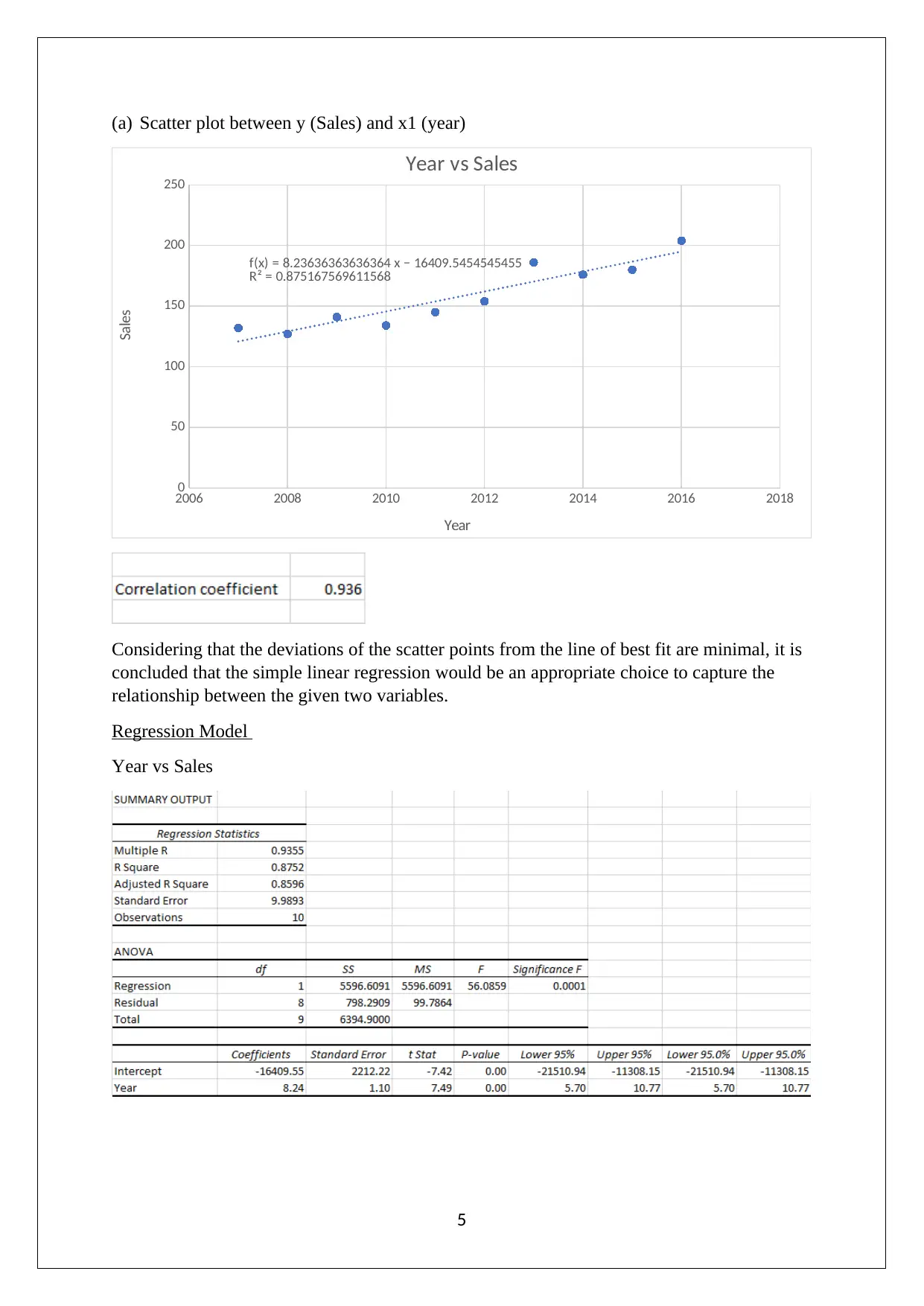
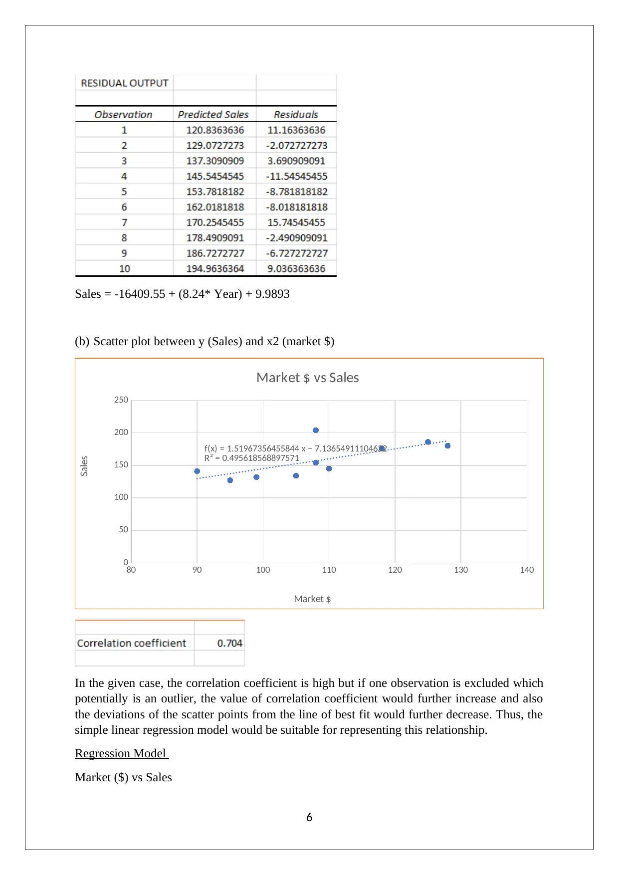
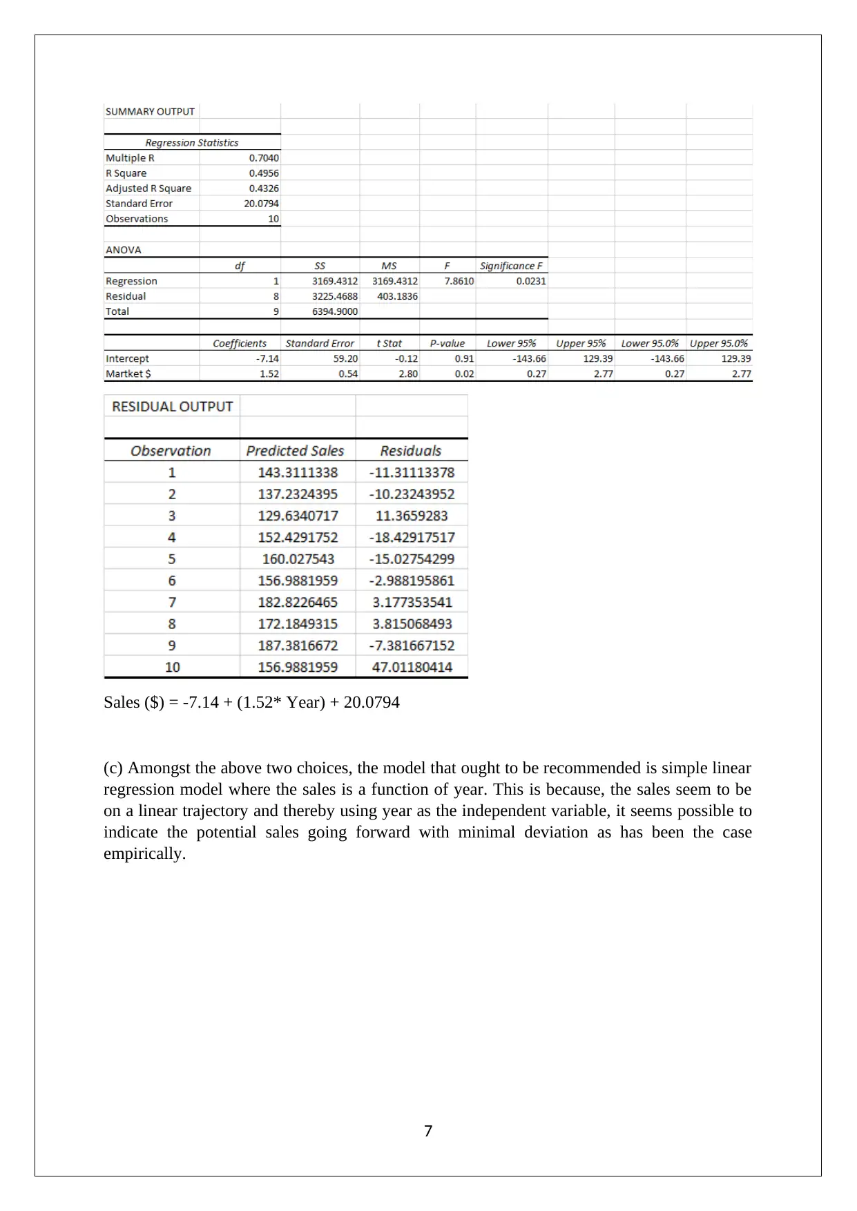
This assignment solution covers various aspects of inventory control systems. Question 1 uses a critical ratio to determine the optimal number of trees to cut. Question 2 calculates the optimal order quantity and reorder level. Question 3 delves into probabilistic models, calculating the reorder point and safety stock with different service levels. Question 4 analyzes the impact of different inventory costing methods (FIFO, LIFO, and weighted average) on profit margins. Finally, question 5 explores regression analysis to model the relationship between sales, years, and market values, recommending a model based on the year for sales forecasting.

INVENTORY CONTROL SYSTEM

Question 1
Selling price P = $30
Cost C = $12
Salvage value G = 0
Shortage or underage cost Cu = P-C = 30-12 =$18
Excess or overstocking cost Co = C- G = 12-0 = $12
Critical ratio = Cu / (Cu + Co) = 18/(18+12) = 0.60
The critical ratio 0.60 falls in the batch number 5.
Batches Probability Cumulative probability Shortage Overage
0
1 0.03 0.03 4
2 0.09 0.12 3
3 0.11 0.23 2
4 0.17 0.40 1
5 0.22 0.62 0 0
6 0.16 0.78 1 0
7 0.13 0.91 2 0
8 0.05 0.96 3 0
9 0.04 1.00 4 0
Therefore, the optimal number of trees to cut Q = 5 Batches = 5*100 = 500 Trees.
Average demand = (1*0.03) +
(2*0.09)+(3*0.11)+(4*0.17)+(5*0.22)+(6*0.16)+(7*0.13)+(8*0.05)+(9*0.04) = 4.95
Expected shortage = (0*0.03) +
(0*0.09)+(0*0.11)+(0*0.17)+(0*0.22)+(1*0.16)+(2*0.13)+(3*0.05)+(4*0.04) = 0.73
Expected sales = Average demand - Expected shortage = 4.95-0.73 = 4.22
Expected overage = 5-4.22 = 0.78
Expected revenue = (30*4.22 + 0.78*0)*100 = $12660
Expected cost = 12*5*100= $6000
Expected profit = 12660 – 6000 = $6660
Question 2
Mean demand = 9.5 units a month
Lead time = 1 month
Shortage cost = $140 a unit a month
1

Reorder cost = $50
Holding cost = $6 a unit a month
Optimal value for order quantity =?
Reorder level =?
Now,
Optimal value for order quantity = Sqrt (2*Demand* Shortage cost /Holding cost)
Optimal value for order quantity = Sqrt (2*9.5*140/6) = 21.05 units
Further,
Reorder point = Demand per day * Lead time = 9.5*1 = 9.5
Question 3
Mean demand = 220 units a week
Standard deviation = 25 units
Constant lead time = 2 weeks
Each unit cost = $7.50 a week to store
Service level = 95%
Reorder cost = $400 per order
Unit cost = $100
This is the probabilistic model where the demand is variable and lead time is constant.
Now,
ROP = (Mean demand * Lead time) + (Z* standard deviation of demand per day* sqrt (Lead
time)
The z value for 95% service level assuming normal distribution = 1.65 (Normal Table)
ROP = (220 * 2) + (1.65*25* sqrt (2))
ROP = 440 + 58.34 = 498.34 or 498
Safety stock = (Z* standard deviation of demand per day* sqrt (Lead time) = (1.65*25* sqrt
(2)) = 58.34 or 58
Therefore, the ROP would be 498 and safety stock would be 58 approximately.
The ABC Company would follow the practice to maintain the ROP as 498 and safety stock as
58.
Total annual cost = (200*100/52)+(298*400) = $11,9584
2

The z value for 98% service level assuming normal distribution = 2.055 (Normal Table)
ROP = (220 * 2) + (2.055*25* sqrt (2))
ROP = 440 + 72.66 = 512.66 or 513
Safety stock = (Z* standard deviation of demand per day* sqrt (Lead time) = (2.055*25* sqrt
(2)) = 72.66 or 73
Therefore, the ROP would be 513 and safety stock would be 73 approximately.
The value of ROP and safety stock has increased as the service level has increased from 95%
to 98%.
Question 4
Total units sold during the six months = 98+84+65+130+82+56 = 515 units
Unit sale price = $40
Total sale revenue = 515*40 = $20,600
The profit and profit margin would depend on the cost of inventory which is a function of the
inventory method deployed.
As per FIFO, the inventory that has been purchased first would also be sold first. The
computation of the cost of goods sold under this method is shown below.
Value of closing stock = 30*28+90*30 = 840+2700 =$3,540
Cost of goods sold = 2450+2162+1586 +3366 + 2228 +1568 =$13,360
Profit = Total sale revenue - Cost of goods sold = 20600 – 13360 = $7,240
Profit margin (%) = (7240/20600)*100 = 35.15%
As per LIFO, the inventory that has been purchased last would also be sold first. The
computation of the cost of goods sold under this method is shown below.
3

Value of closing stock = 20*27 + 35*24 + 13*25 + 18*28 + 34*30 =$3,229
Cost of goods sold = 2450+2175+1560 +3510 + 2296 +1680 =$13,671
Profit = Total sale revenue - Cost of goods sold = 20600 – 13671 = $6,929
Profit margin (%) = (6929/20600)*100 = 33.62%
As per weighted average, the inventory that has been purchased would be sold at the
weighted average cost of inventory available for sale. The computation of the cost of goods
sold under this method is shown below.
Value of closing stock = 120*26.67 = $3200.4
Cost of goods sold = 2450+2164.95+1573.26 +3421.88+1900.87+1493.52 =$13,004.48
Profit = Total sale revenue - Cost of goods sold = 20600 – 13004.48 = $7595.52
Profit margin (%) = (7595.52/20600)*100 = 36.87%
Question 5
4

(a) Scatter plot between y (Sales) and x1 (year)
2006 2008 2010 2012 2014 2016 2018
0
50
100
150
200
250
f(x) = 8.23636363636364 x − 16409.5454545455
R² = 0.875167569611568
Year vs Sales
Year
Sales
Considering that the deviations of the scatter points from the line of best fit are minimal, it is
concluded that the simple linear regression would be an appropriate choice to capture the
relationship between the given two variables.
Regression Model
Year vs Sales
5

Sales = -16409.55 + (8.24* Year) + 9.9893
(b) Scatter plot between y (Sales) and x2 (market $)
80 90 100 110 120 130 140
0
50
100
150
200
250
f(x) = 1.51967356455844 x − 7.13654911104632
R² = 0.495618568897571
Market $ vs Sales
Market $
Sales
In the given case, the correlation coefficient is high but if one observation is excluded which
potentially is an outlier, the value of correlation coefficient would further increase and also
the deviations of the scatter points from the line of best fit would further decrease. Thus, the
simple linear regression model would be suitable for representing this relationship.
Regression Model
Market ($) vs Sales
6

Sales ($) = -7.14 + (1.52* Year) + 20.0794
(c) Amongst the above two choices, the model that ought to be recommended is simple linear
regression model where the sales is a function of year. This is because, the sales seem to be
on a linear trajectory and thereby using year as the independent variable, it seems possible to
indicate the potential sales going forward with minimal deviation as has been the case
empirically.
7