Analysis of Inventory Costing and Depreciation Methods in Accounting
VerifiedAdded on 2020/03/23
|14
|3321
|67
Practical Assignment
AI Summary
This assignment solution comprehensively addresses inventory costing and depreciation methods. Part A calculates the cost of inventory at a specific date using both the FIFO and moving average methods, providing detailed calculations and balances. Part B focuses on journal entries to account for inventory shrinkage under both costing methods. Part C delves into sales, cost of sales, and inventory ledger accounts using the moving average method. Solution 2 explores depreciation, offering schedules for straight-line, diminishing balance, sum of years' digits, and units-of-production methods. It also compares these methods, providing advantages, disadvantages, and recommendations for method selection based on AASB 116. The analysis includes profit calculations under each method, supporting the recommendation of the units of production method. Solution 3 presents ledger accounts for machine transactions, detailing the impact of purchases, sales, and depreciation on the machine's value.
Solution-1
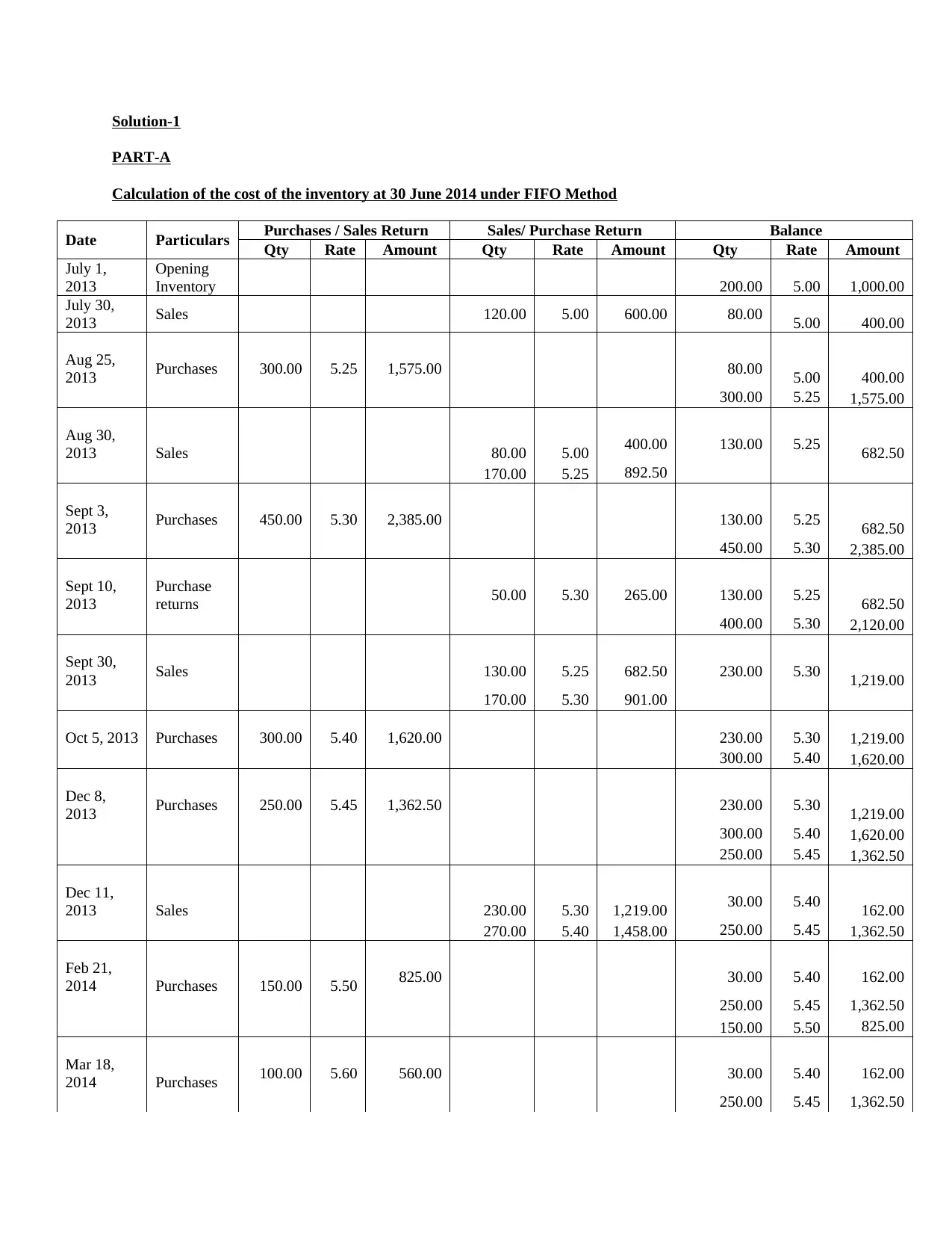
PART-A
Calculation of the cost of the inventory at 30 June 2014 under FIFO Method
Date Particulars Purchases / Sales Return Sales/ Purchase Return Balance
Qty Rate Amount Qty Rate Amount Qty Rate Amount
July 1,
2013
Opening
Inventory 200.00 5.00 1,000.00
July 30,
2013 Sales 120.00 5.00 600.00 80.00 5.00 400.00
Aug 25,
2013 Purchases 300.00 5.25 1,575.00 80.00 5.00 400.00
300.00 5.25 1,575.00
Aug 30,
2013 Sales 80.00 5.00 400.00 130.00 5.25 682.50
170.00 5.25 892.50
Sept 3,
2013 Purchases 450.00 5.30 2,385.00 130.00 5.25 682.50
450.00 5.30 2,385.00
Sept 10,
2013
Purchase
returns 50.00 5.30 265.00 130.00 5.25 682.50
400.00 5.30 2,120.00
Sept 30,
2013 Sales 130.00 5.25 682.50 230.00 5.30 1,219.00
170.00 5.30 901.00
Oct 5, 2013 Purchases 300.00 5.40 1,620.00 230.00 5.30 1,219.00
300.00 5.40 1,620.00
Dec 8,
2013 Purchases 250.00 5.45 1,362.50 230.00 5.30 1,219.00
300.00 5.40 1,620.00
250.00 5.45 1,362.50
Dec 11,
2013 Sales 230.00 5.30 1,219.00 30.00 5.40 162.00
270.00 5.40 1,458.00 250.00 5.45 1,362.50
Feb 21,
2014 Purchases 150.00 5.50 825.00 30.00 5.40 162.00
250.00 5.45 1,362.50
150.00 5.50 825.00
Mar 18,
2014 Purchases 100.00 5.60 560.00 30.00 5.40 162.00
250.00 5.45 1,362.50
Paraphrase This Document
Need a fresh take? Get an instant paraphrase of this document with our AI Paraphraser
150.00 5.50 825.00
100.00 5.60 560.00
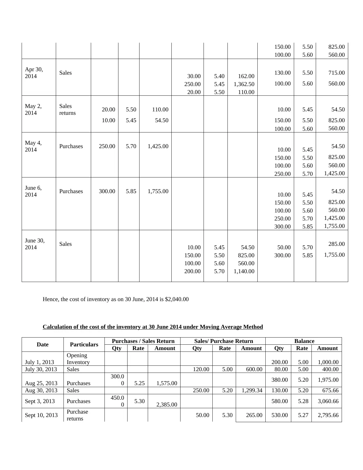
Apr 30,
2014 Sales 30.00 5.40 162.00 130.00 5.50 715.00
250.00 5.45 1,362.50 100.00 5.60 560.00
20.00 5.50 110.00
May 2,
2014
Sales
returns 20.00 5.50 110.00 10.00 5.45 54.50
10.00 5.45 54.50 150.00 5.50 825.00
100.00 5.60 560.00
May 4,
2014 Purchases 250.00 5.70 1,425.00 10.00 5.45 54.50
150.00 5.50 825.00
100.00 5.60 560.00
250.00 5.70 1,425.00
June 6,
2014 Purchases 300.00 5.85 1,755.00 10.00 5.45 54.50
150.00 5.50 825.00
100.00 5.60 560.00
250.00 5.70 1,425.00
300.00 5.85 1,755.00
June 30,
2014 Sales 10.00 5.45 54.50 50.00 5.70 285.00
150.00 5.50 825.00 300.00 5.85 1,755.00
100.00 5.60 560.00
200.00 5.70 1,140.00
Hence, the cost of inventory as on 30 June, 2014 is $2,040.00
Calculation of the cost of the inventory at 30 June 2014 under Moving Average Method
Date Particulars Purchases / Sales Return Sales/ Purchase Return Balance
Qty Rate Amount Qty Rate Amount Qty Rate Amount
July 1, 2013
Opening
Inventory 200.00 5.00 1,000.00
July 30, 2013 Sales 120.00 5.00 600.00 80.00 5.00 400.00
Aug 25, 2013 Purchases
300.0
0 5.25 1,575.00 380.00 5.20 1,975.00
Aug 30, 2013 Sales 250.00 5.20 1,299.34 130.00 5.20 675.66
Sept 3, 2013 Purchases 450.0
0 5.30 2,385.00 580.00 5.28 3,060.66
Sept 10, 2013 Purchase
returns 50.00 5.30 265.00 530.00 5.27 2,795.66
100.00 5.60 560.00
Apr 30,
2014 Sales 30.00 5.40 162.00 130.00 5.50 715.00
250.00 5.45 1,362.50 100.00 5.60 560.00
20.00 5.50 110.00
May 2,
2014
Sales
returns 20.00 5.50 110.00 10.00 5.45 54.50
10.00 5.45 54.50 150.00 5.50 825.00
100.00 5.60 560.00
May 4,
2014 Purchases 250.00 5.70 1,425.00 10.00 5.45 54.50
150.00 5.50 825.00
100.00 5.60 560.00
250.00 5.70 1,425.00
June 6,
2014 Purchases 300.00 5.85 1,755.00 10.00 5.45 54.50
150.00 5.50 825.00
100.00 5.60 560.00
250.00 5.70 1,425.00
300.00 5.85 1,755.00
June 30,
2014 Sales 10.00 5.45 54.50 50.00 5.70 285.00
150.00 5.50 825.00 300.00 5.85 1,755.00
100.00 5.60 560.00
200.00 5.70 1,140.00
Hence, the cost of inventory as on 30 June, 2014 is $2,040.00
Calculation of the cost of the inventory at 30 June 2014 under Moving Average Method
Date Particulars Purchases / Sales Return Sales/ Purchase Return Balance
Qty Rate Amount Qty Rate Amount Qty Rate Amount
July 1, 2013
Opening
Inventory 200.00 5.00 1,000.00
July 30, 2013 Sales 120.00 5.00 600.00 80.00 5.00 400.00
Aug 25, 2013 Purchases
300.0
0 5.25 1,575.00 380.00 5.20 1,975.00
Aug 30, 2013 Sales 250.00 5.20 1,299.34 130.00 5.20 675.66
Sept 3, 2013 Purchases 450.0
0 5.30 2,385.00 580.00 5.28 3,060.66
Sept 10, 2013 Purchase
returns 50.00 5.30 265.00 530.00 5.27 2,795.66
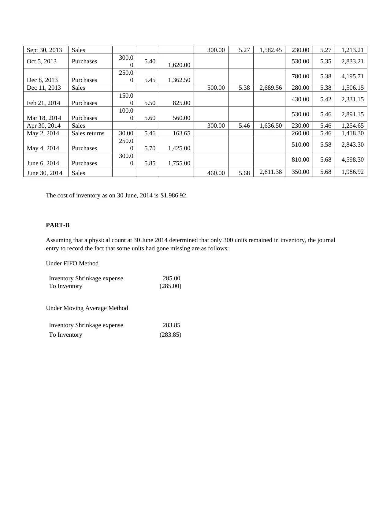
Sept 30, 2013 Sales 300.00 5.27 1,582.45 230.00 5.27 1,213.21
Oct 5, 2013 Purchases 300.0
0 5.40 1,620.00 530.00 5.35 2,833.21
Dec 8, 2013 Purchases
250.0
0 5.45 1,362.50 780.00 5.38 4,195.71
Dec 11, 2013 Sales 500.00 5.38 2,689.56 280.00 5.38 1,506.15
Feb 21, 2014 Purchases
150.0
0 5.50 825.00 430.00 5.42 2,331.15
Mar 18, 2014 Purchases
100.0
0 5.60 560.00 530.00 5.46 2,891.15
Apr 30, 2014 Sales 300.00 5.46 1,636.50 230.00 5.46 1,254.65
May 2, 2014 Sales returns 30.00 5.46 163.65 260.00 5.46 1,418.30
May 4, 2014 Purchases
250.0
0 5.70 1,425.00 510.00 5.58 2,843.30
June 6, 2014 Purchases
300.0
0 5.85 1,755.00 810.00 5.68 4,598.30
June 30, 2014 Sales 460.00 5.68 2,611.38 350.00 5.68 1,986.92
The cost of inventory as on 30 June, 2014 is $1,986.92.
PART-B
Assuming that a physical count at 30 June 2014 determined that only 300 units remained in inventory, the journal
entry to record the fact that some units had gone missing are as follows:
Under FIFO Method
Inventory Shrinkage expense 285.00
To Inventory (285.00)
Under Moving Average Method
Inventory Shrinkage expense 283.85
To Inventory (283.85)
⊘ This is a preview!⊘
Do you want full access?
Subscribe today to unlock all pages.
Trusted by 1+ million students worldwide
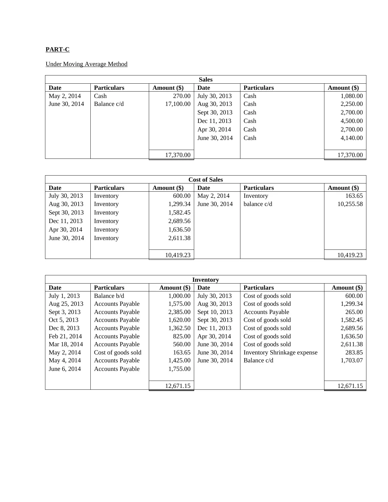
PART-C
Under Moving Average Method
Sales
Date Particulars Amount ($) Date Particulars Amount ($)
May 2, 2014 Cash 270.00 July 30, 2013 Cash 1,080.00
June 30, 2014 Balance c/d 17,100.00 Aug 30, 2013 Cash 2,250.00
Sept 30, 2013 Cash 2,700.00
Dec 11, 2013 Cash 4,500.00
Apr 30, 2014 Cash 2,700.00
June 30, 2014 Cash 4,140.00
17,370.00 17,370.00
Cost of Sales
Date Particulars Amount ($) Date Particulars Amount ($)
July 30, 2013 Inventory 600.00 May 2, 2014 Inventory 163.65
Aug 30, 2013 Inventory 1,299.34 June 30, 2014 balance c/d 10,255.58
Sept 30, 2013 Inventory 1,582.45
Dec 11, 2013 Inventory 2,689.56
Apr 30, 2014 Inventory 1,636.50
June 30, 2014 Inventory 2,611.38
10,419.23 10,419.23
Inventory
Date Particulars Amount ($) Date Particulars Amount ($)
July 1, 2013 Balance b/d 1,000.00 July 30, 2013 Cost of goods sold 600.00
Aug 25, 2013 Accounts Payable 1,575.00 Aug 30, 2013 Cost of goods sold 1,299.34
Sept 3, 2013 Accounts Payable 2,385.00 Sept 10, 2013 Accounts Payable 265.00
Oct 5, 2013 Accounts Payable 1,620.00 Sept 30, 2013 Cost of goods sold 1,582.45
Dec 8, 2013 Accounts Payable 1,362.50 Dec 11, 2013 Cost of goods sold 2,689.56
Feb 21, 2014 Accounts Payable 825.00 Apr 30, 2014 Cost of goods sold 1,636.50
Mar 18, 2014 Accounts Payable 560.00 June 30, 2014 Cost of goods sold 2,611.38
May 2, 2014 Cost of goods sold 163.65 June 30, 2014 Inventory Shrinkage expense 283.85
May 4, 2014 Accounts Payable 1,425.00 June 30, 2014 Balance c/d 1,703.07
June 6, 2014 Accounts Payable 1,755.00
12,671.15 12,671.15
Paraphrase This Document
Need a fresh take? Get an instant paraphrase of this document with our AI Paraphraser
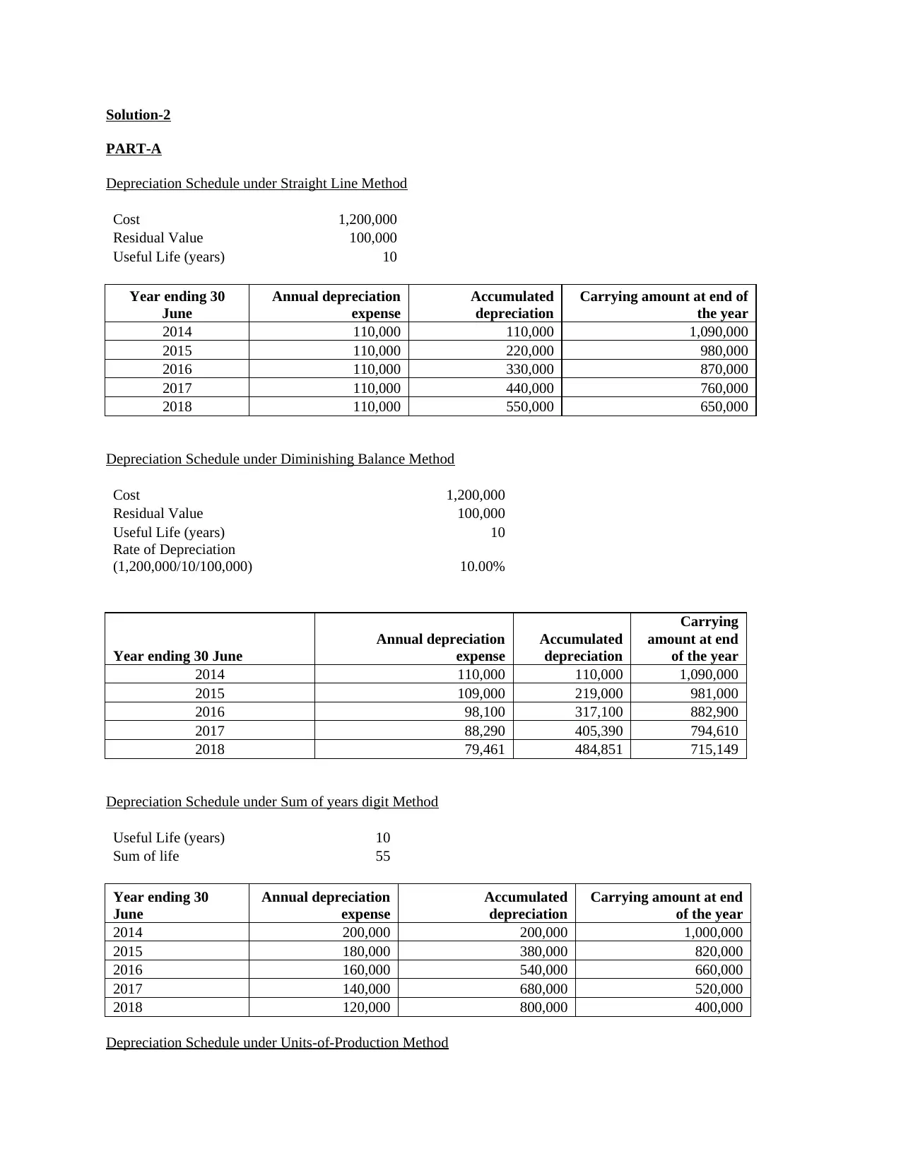
Solution-2
PART-A
Depreciation Schedule under Straight Line Method
Cost 1,200,000
Residual Value 100,000
Useful Life (years) 10
Year ending 30
June
Annual depreciation
expense
Accumulated
depreciation
Carrying amount at end of
the year
2014 110,000 110,000 1,090,000
2015 110,000 220,000 980,000
2016 110,000 330,000 870,000
2017 110,000 440,000 760,000
2018 110,000 550,000 650,000
Depreciation Schedule under Diminishing Balance Method
Cost 1,200,000
Residual Value 100,000
Useful Life (years) 10
Rate of Depreciation
(1,200,000/10/100,000) 10.00%
Year ending 30 June
Annual depreciation
expense
Accumulated
depreciation
Carrying
amount at end
of the year
2014 110,000 110,000 1,090,000
2015 109,000 219,000 981,000
2016 98,100 317,100 882,900
2017 88,290 405,390 794,610
2018 79,461 484,851 715,149
Depreciation Schedule under Sum of years digit Method
Useful Life (years) 10
Sum of life 55
Year ending 30
June
Annual depreciation
expense
Accumulated
depreciation
Carrying amount at end
of the year
2014 200,000 200,000 1,000,000
2015 180,000 380,000 820,000
2016 160,000 540,000 660,000
2017 140,000 680,000 520,000
2018 120,000 800,000 400,000
Depreciation Schedule under Units-of-Production Method
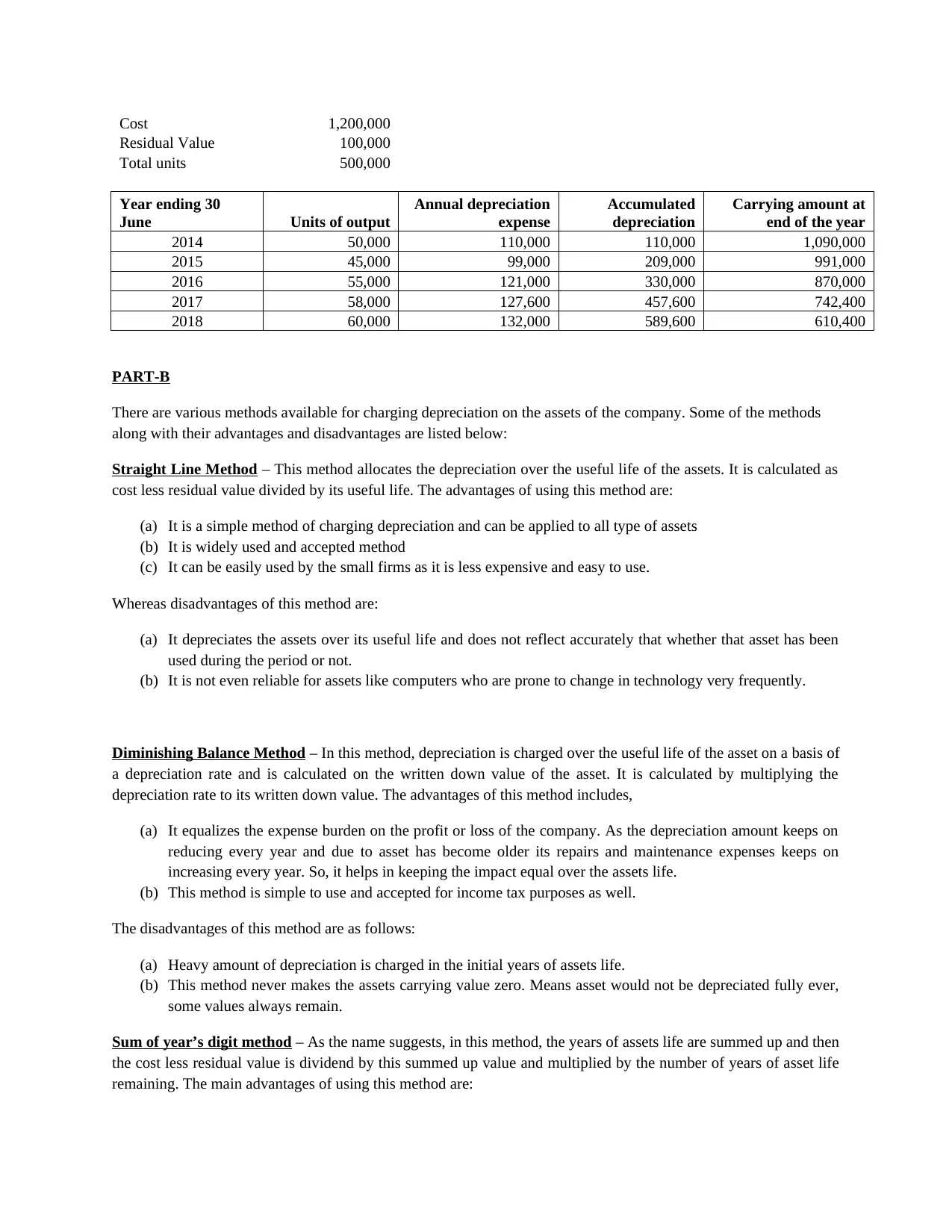
Cost 1,200,000
Residual Value 100,000
Total units 500,000
Year ending 30
June Units of output
Annual depreciation
expense
Accumulated
depreciation
Carrying amount at
end of the year
2014 50,000 110,000 110,000 1,090,000
2015 45,000 99,000 209,000 991,000
2016 55,000 121,000 330,000 870,000
2017 58,000 127,600 457,600 742,400
2018 60,000 132,000 589,600 610,400
PART-B
There are various methods available for charging depreciation on the assets of the company. Some of the methods
along with their advantages and disadvantages are listed below:
Straight Line Method – This method allocates the depreciation over the useful life of the assets. It is calculated as
cost less residual value divided by its useful life. The advantages of using this method are:
(a) It is a simple method of charging depreciation and can be applied to all type of assets
(b) It is widely used and accepted method
(c) It can be easily used by the small firms as it is less expensive and easy to use.
Whereas disadvantages of this method are:
(a) It depreciates the assets over its useful life and does not reflect accurately that whether that asset has been
used during the period or not.
(b) It is not even reliable for assets like computers who are prone to change in technology very frequently.
Diminishing Balance Method – In this method, depreciation is charged over the useful life of the asset on a basis of
a depreciation rate and is calculated on the written down value of the asset. It is calculated by multiplying the
depreciation rate to its written down value. The advantages of this method includes,
(a) It equalizes the expense burden on the profit or loss of the company. As the depreciation amount keeps on
reducing every year and due to asset has become older its repairs and maintenance expenses keeps on
increasing every year. So, it helps in keeping the impact equal over the assets life.
(b) This method is simple to use and accepted for income tax purposes as well.
The disadvantages of this method are as follows:
(a) Heavy amount of depreciation is charged in the initial years of assets life.
(b) This method never makes the assets carrying value zero. Means asset would not be depreciated fully ever,
some values always remain.
Sum of year’s digit method – As the name suggests, in this method, the years of assets life are summed up and then
the cost less residual value is dividend by this summed up value and multiplied by the number of years of asset life
remaining. The main advantages of using this method are:
⊘ This is a preview!⊘
Do you want full access?
Subscribe today to unlock all pages.
Trusted by 1+ million students worldwide
(a) This method matches the revenue with expenses, as the depreciation is higher in the initial years and low
in the last years.
(b) It accurately reflects the difference in the usage of the assets from one year to another.
The disadvantages are as below:
(a) The depreciation is higher in initial years irrespective of usage of assets.
(b) This method is quite confusing and baseless.
Units of production Method – In this method, the depreciation is charged on the basis of number of units produced
by the asset. It is calculated by dividing the cost of the assets less residual value with the total number of units
expected to be produced over the life of the asset multiplied by the number of units produced in the given period or
year. The advantages of this method are:
(a) It is more scientific method as it allocates the depreciation on the basis future economic benefits expected
to be received from the asset.
(b) This method matches the revenue and expense concept. As more units produced the revenue will be higher
and the depreciation will also be in the ratio of units produced.
The disadvantages are:
(a) There will be no depreciation if the asset has not produced any units irrespective of the fact that the asset is
losing its value day by day by the passage of time.
(b) This method can be applied only on assets involved in production; other assets like building etc. can’t be
depreciated using this method.
Standard’s Perception - As per AASB 116, the depreciation method adopted by the company should be related to the
future economic benefits provided by the asset. The AASB recognizes the straight line method, diminishing value
method and units of production method. But the sum of year’s digit method is not recognized by the standard and
hence can’t be used.
Recommendations - We recommend the management to use units of production method, as this method is clearly
related to the future economic benefits provided by the asset. It allocates the depreciation on the basis of number of
units produced and the units produced will give the benefit in terms of generating revenue.
The net profits after depreciation under different methods are as below:
Straight Line Method
Year ending
30 June
Profit before
depreciation Depreciation
Profit after
depreciation
2014 350,000 110,000 240,000
2015 340,000 110,000 230,000
2016 355,000 110,000 245,000
2017 360,000 110,000 250,000
2018 380,000 110,000 270,000
Diminishing Balance Method
Paraphrase This Document
Need a fresh take? Get an instant paraphrase of this document with our AI Paraphraser
Year ending
30 June
Profit before
depreciation Depreciation
Profit after
depreciation
2014 350,000 110,000 240,000
2015 340,000 109,000 231,000
2016 355,000 98,100 256,900
2017 360,000 88,290 271,710
2018 380,000 79,461 300,539
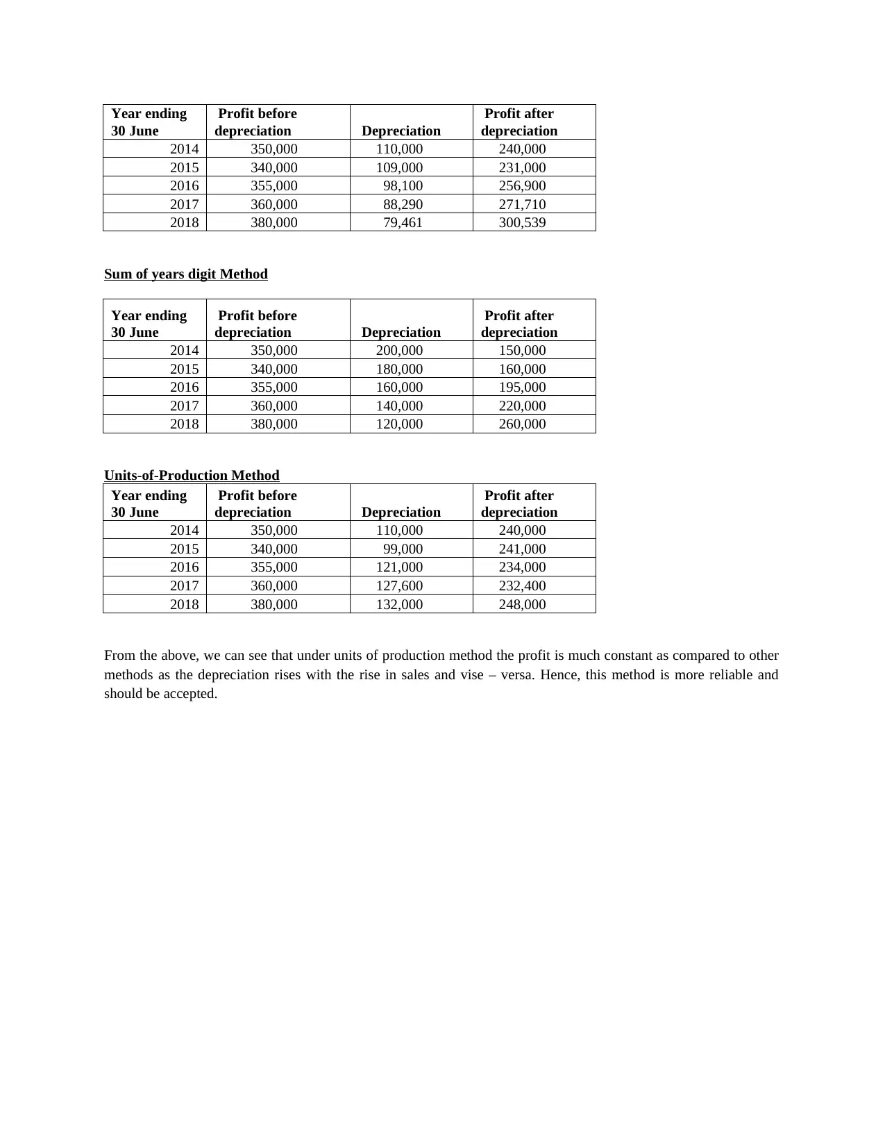
Sum of years digit Method
Year ending
30 June
Profit before
depreciation Depreciation
Profit after
depreciation
2014 350,000 200,000 150,000
2015 340,000 180,000 160,000
2016 355,000 160,000 195,000
2017 360,000 140,000 220,000
2018 380,000 120,000 260,000
Units-of-Production Method
Year ending
30 June
Profit before
depreciation Depreciation
Profit after
depreciation
2014 350,000 110,000 240,000
2015 340,000 99,000 241,000
2016 355,000 121,000 234,000
2017 360,000 127,600 232,400
2018 380,000 132,000 248,000
From the above, we can see that under units of production method the profit is much constant as compared to other
methods as the depreciation rises with the rise in sales and vise – versa. Hence, this method is more reliable and
should be accepted.
30 June
Profit before
depreciation Depreciation
Profit after
depreciation
2014 350,000 110,000 240,000
2015 340,000 109,000 231,000
2016 355,000 98,100 256,900
2017 360,000 88,290 271,710
2018 380,000 79,461 300,539
Sum of years digit Method
Year ending
30 June
Profit before
depreciation Depreciation
Profit after
depreciation
2014 350,000 200,000 150,000
2015 340,000 180,000 160,000
2016 355,000 160,000 195,000
2017 360,000 140,000 220,000
2018 380,000 120,000 260,000
Units-of-Production Method
Year ending
30 June
Profit before
depreciation Depreciation
Profit after
depreciation
2014 350,000 110,000 240,000
2015 340,000 99,000 241,000
2016 355,000 121,000 234,000
2017 360,000 127,600 232,400
2018 380,000 132,000 248,000
From the above, we can see that under units of production method the profit is much constant as compared to other
methods as the depreciation rises with the rise in sales and vise – versa. Hence, this method is more reliable and
should be accepted.
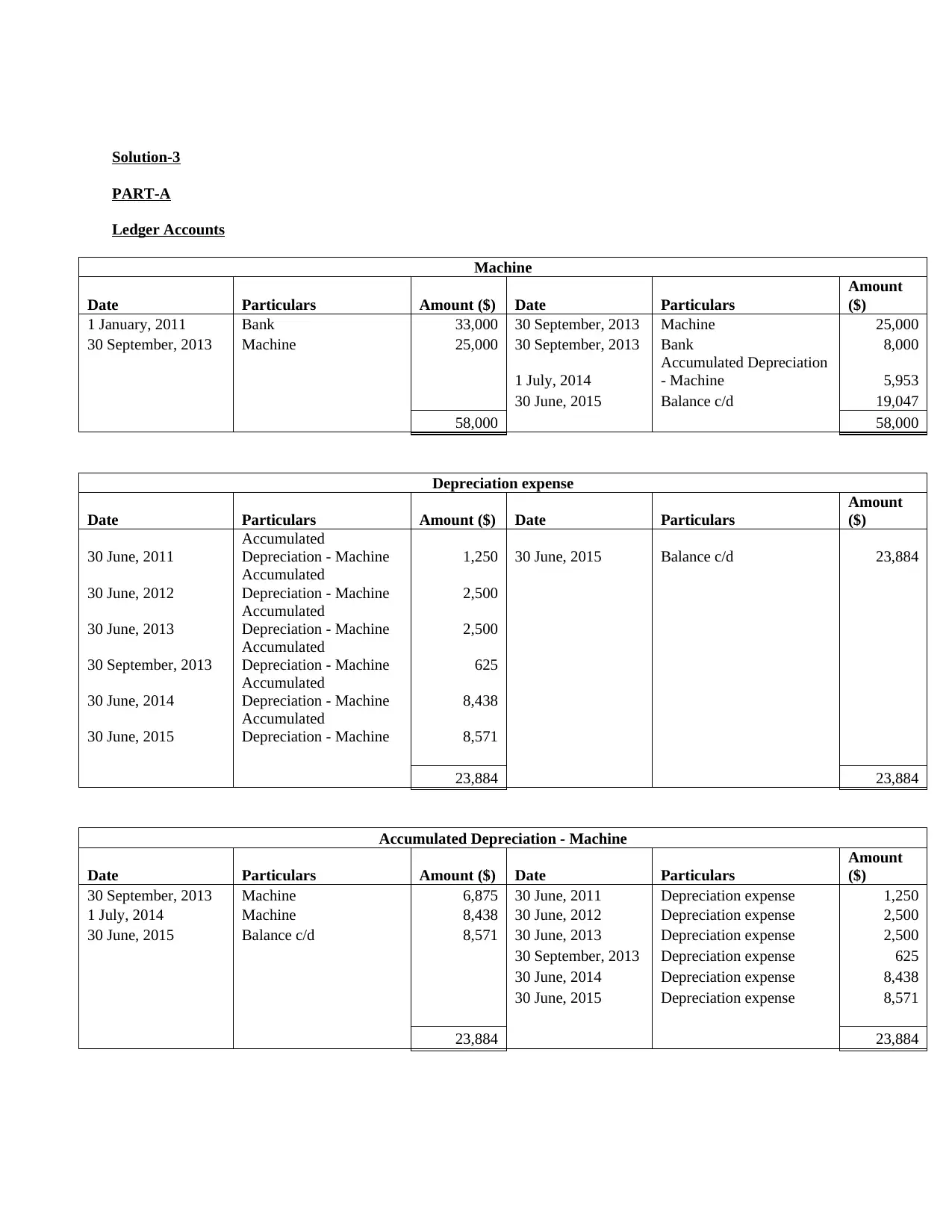
Solution-3
PART-A
Ledger Accounts
Machine
Date Particulars Amount ($) Date Particulars
Amount
($)
1 January, 2011 Bank 33,000 30 September, 2013 Machine 25,000
30 September, 2013 Machine 25,000 30 September, 2013 Bank 8,000
1 July, 2014
Accumulated Depreciation
- Machine 5,953
30 June, 2015 Balance c/d 19,047
58,000 58,000
Depreciation expense
Date Particulars Amount ($) Date Particulars
Amount
($)
30 June, 2011
Accumulated
Depreciation - Machine 1,250 30 June, 2015 Balance c/d 23,884
30 June, 2012
Accumulated
Depreciation - Machine 2,500
30 June, 2013
Accumulated
Depreciation - Machine 2,500
30 September, 2013
Accumulated
Depreciation - Machine 625
30 June, 2014
Accumulated
Depreciation - Machine 8,438
30 June, 2015
Accumulated
Depreciation - Machine 8,571
23,884 23,884
Accumulated Depreciation - Machine
Date Particulars Amount ($) Date Particulars
Amount
($)
30 September, 2013 Machine 6,875 30 June, 2011 Depreciation expense 1,250
1 July, 2014 Machine 8,438 30 June, 2012 Depreciation expense 2,500
30 June, 2015 Balance c/d 8,571 30 June, 2013 Depreciation expense 2,500
30 September, 2013 Depreciation expense 625
30 June, 2014 Depreciation expense 8,438
30 June, 2015 Depreciation expense 8,571
23,884 23,884
⊘ This is a preview!⊘
Do you want full access?
Subscribe today to unlock all pages.
Trusted by 1+ million students worldwide
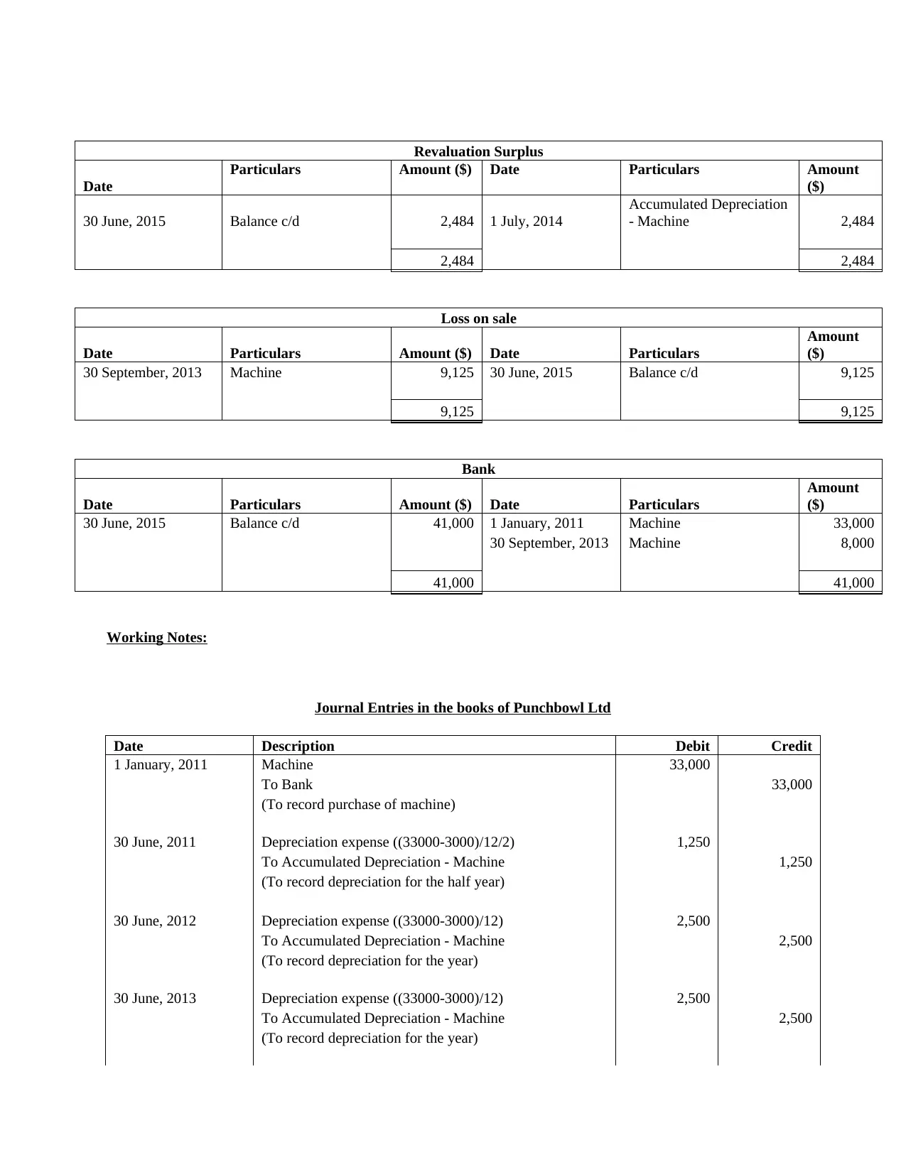
Revaluation Surplus
Date
Particulars Amount ($) Date Particulars Amount
($)
30 June, 2015 Balance c/d 2,484 1 July, 2014
Accumulated Depreciation
- Machine 2,484
2,484 2,484
Loss on sale
Date Particulars Amount ($) Date Particulars
Amount
($)
30 September, 2013 Machine 9,125 30 June, 2015 Balance c/d 9,125
9,125 9,125
Bank
Date Particulars Amount ($) Date Particulars
Amount
($)
30 June, 2015 Balance c/d 41,000 1 January, 2011 Machine 33,000
30 September, 2013 Machine 8,000
41,000 41,000
Working Notes:
Journal Entries in the books of Punchbowl Ltd
Date Description Debit Credit
1 January, 2011 Machine 33,000
To Bank 33,000
(To record purchase of machine)
30 June, 2011 Depreciation expense ((33000-3000)/12/2) 1,250
To Accumulated Depreciation - Machine 1,250
(To record depreciation for the half year)
30 June, 2012 Depreciation expense ((33000-3000)/12) 2,500
To Accumulated Depreciation - Machine 2,500
(To record depreciation for the year)
30 June, 2013 Depreciation expense ((33000-3000)/12) 2,500
To Accumulated Depreciation - Machine 2,500
(To record depreciation for the year)
Paraphrase This Document
Need a fresh take? Get an instant paraphrase of this document with our AI Paraphraser
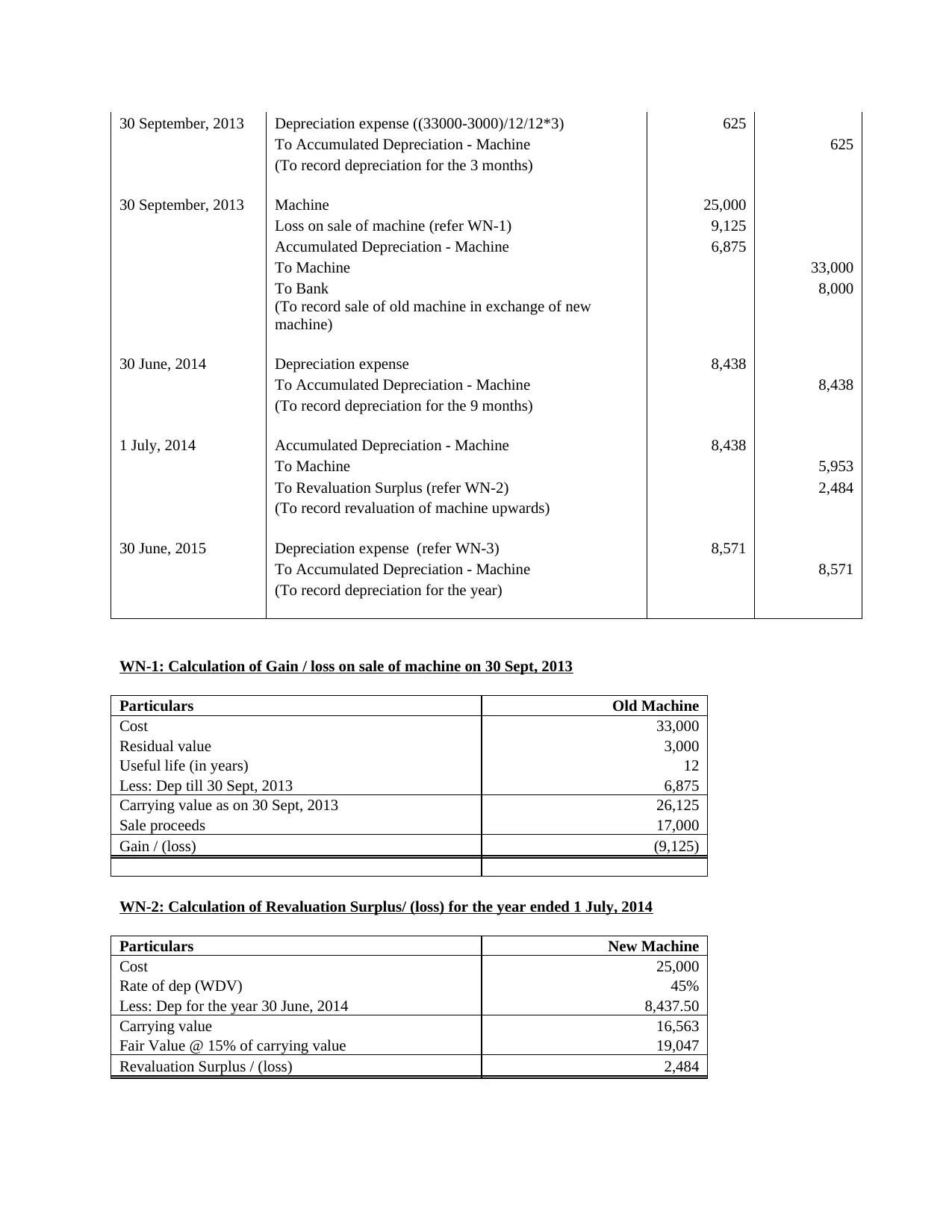
30 September, 2013 Depreciation expense ((33000-3000)/12/12*3) 625
To Accumulated Depreciation - Machine 625
(To record depreciation for the 3 months)
30 September, 2013 Machine 25,000
Loss on sale of machine (refer WN-1) 9,125
Accumulated Depreciation - Machine 6,875
To Machine 33,000
To Bank 8,000
(To record sale of old machine in exchange of new
machine)
30 June, 2014 Depreciation expense 8,438
To Accumulated Depreciation - Machine 8,438
(To record depreciation for the 9 months)
1 July, 2014 Accumulated Depreciation - Machine 8,438
To Machine 5,953
To Revaluation Surplus (refer WN-2) 2,484
(To record revaluation of machine upwards)
30 June, 2015 Depreciation expense (refer WN-3) 8,571
To Accumulated Depreciation - Machine 8,571
(To record depreciation for the year)
WN-1: Calculation of Gain / loss on sale of machine on 30 Sept, 2013
Particulars Old Machine
Cost 33,000
Residual value 3,000
Useful life (in years) 12
Less: Dep till 30 Sept, 2013 6,875
Carrying value as on 30 Sept, 2013 26,125
Sale proceeds 17,000
Gain / (loss) (9,125)
WN-2: Calculation of Revaluation Surplus/ (loss) for the year ended 1 July, 2014
Particulars New Machine
Cost 25,000
Rate of dep (WDV) 45%
Less: Dep for the year 30 June, 2014 8,437.50
Carrying value 16,563
Fair Value @ 15% of carrying value 19,047
Revaluation Surplus / (loss) 2,484
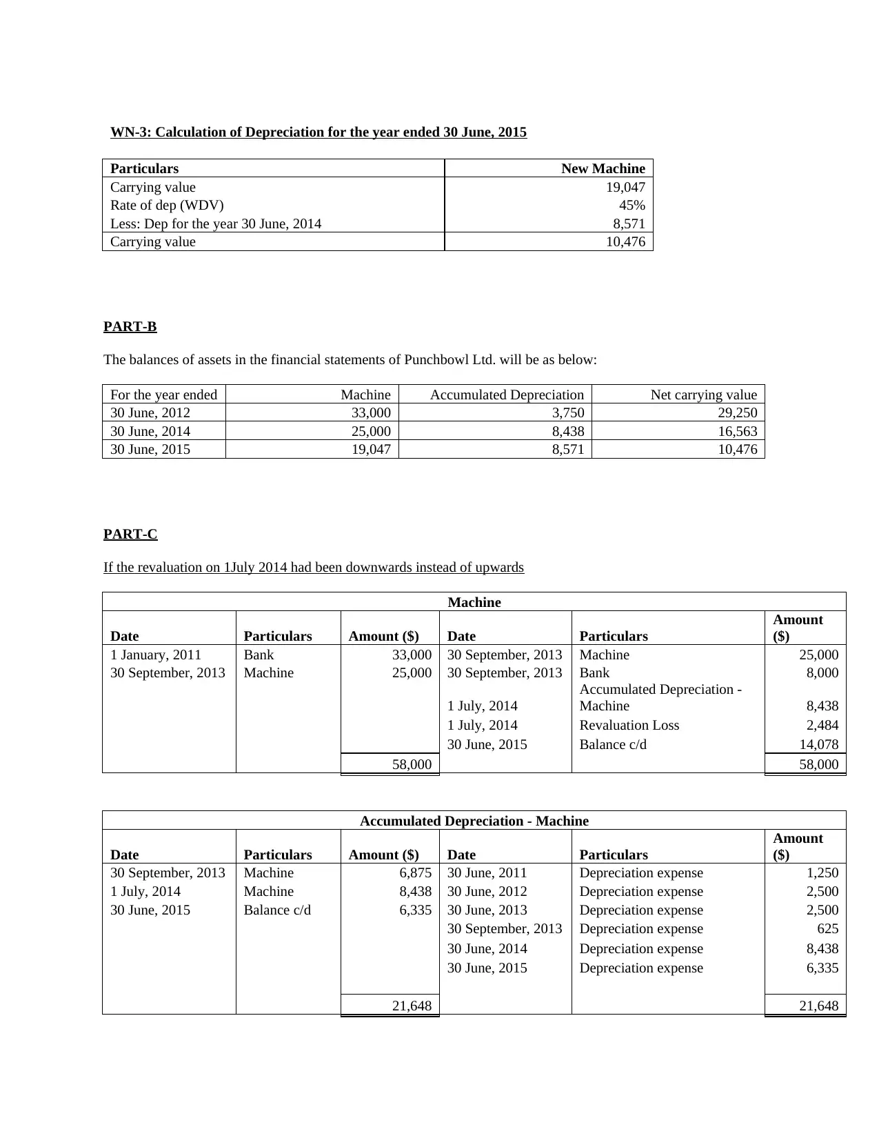
WN-3: Calculation of Depreciation for the year ended 30 June, 2015
Particulars New Machine
Carrying value 19,047
Rate of dep (WDV) 45%
Less: Dep for the year 30 June, 2014 8,571
Carrying value 10,476
PART-B
The balances of assets in the financial statements of Punchbowl Ltd. will be as below:
For the year ended Machine Accumulated Depreciation Net carrying value
30 June, 2012 33,000 3,750 29,250
30 June, 2014 25,000 8,438 16,563
30 June, 2015 19,047 8,571 10,476
PART-C
If the revaluation on 1July 2014 had been downwards instead of upwards
Machine
Date Particulars Amount ($) Date Particulars
Amount
($)
1 January, 2011 Bank 33,000 30 September, 2013 Machine 25,000
30 September, 2013 Machine 25,000 30 September, 2013 Bank 8,000
1 July, 2014
Accumulated Depreciation -
Machine 8,438
1 July, 2014 Revaluation Loss 2,484
30 June, 2015 Balance c/d 14,078
58,000 58,000
Accumulated Depreciation - Machine
Date Particulars Amount ($) Date Particulars
Amount
($)
30 September, 2013 Machine 6,875 30 June, 2011 Depreciation expense 1,250
1 July, 2014 Machine 8,438 30 June, 2012 Depreciation expense 2,500
30 June, 2015 Balance c/d 6,335 30 June, 2013 Depreciation expense 2,500
30 September, 2013 Depreciation expense 625
30 June, 2014 Depreciation expense 8,438
30 June, 2015 Depreciation expense 6,335
21,648 21,648
⊘ This is a preview!⊘
Do you want full access?
Subscribe today to unlock all pages.
Trusted by 1+ million students worldwide
1 out of 14

Your All-in-One AI-Powered Toolkit for Academic Success.
+13062052269
info@desklib.com
Available 24*7 on WhatsApp / Email
![[object Object]](/_next/static/media/star-bottom.7253800d.svg)
Unlock your academic potential
Copyright © 2020–2026 A2Z Services. All Rights Reserved. Developed and managed by ZUCOL.