Inventory Management and Control: Decision Analysis & Valuation

This assignment solution covers key aspects of inventory management and control, including decision analysis, economic order quantity (EOQ) calculations, and inventory control strategies. It delves into inventory valuation methods such as FIFO, LIFO, and weighted average cost, providing detailed calculations and profit analyses for each. Furthermore, the solution incorporates linear regression analysis to forecast sales based on historical data, examining the relationship between sales and both year and market spending. The document includes tables and figures to illustrate the analysis and calculations, offering a comprehensive understanding of the concepts and their practical applications. The solution provides a detailed step-by-step guide to each section of the assignment, including the formulas and calculations used to arrive at the results.

Inventory Management and Control
Course Name:
University:
Student Name:
Student Number:
Section:
Submission Date:

Table of Contents
1. Decision analysis...........................................................................................................3
2. Economic order quantity................................................................................................3
3. Inventory control............................................................................................................5
4. Inventory valuation.........................................................................................................7
5. Linear Regression........................................................................................................10
5.a Y (sales) versus X (year).......................................................................................10
5.b Y (sales) versus X (market$).................................................................................12
List of Figures
Figure 1: Scatter plot of Y (sales) versus X (year)..........................................................11
Figure 2: Scatter plot of Y (sales) versus X (market$)....................................................13
List of Tables
Table 1: Payoff table for decision analysis........................................................................4
Table 2: Inventory valuation (FIFO) and profit calculation................................................8
Table 3: Inventory valuation (LIFO) and profit calculation.................................................9
Table 4: Inventory valuation (Weighted Cost) and profit calculation...............................10
Table 5: least square point estimates for Y (sales) versus X (year)...............................12
Table 6: least square point estimates for Y (sales) versus X (market$).........................14

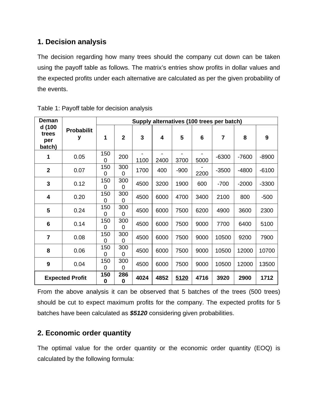
1. Decision analysis
The decision regarding how many trees should the company cut down can be taken
using the payoff table as follows. The matrix’s entries show profits in dollar values and
the expected profits under each alternative are calculated as per the given probability of
the events.
Table 1: Payoff table for decision analysis
Deman
d (100
trees
per
batch)
Probabilit
y
Supply alternatives (100 trees per batch)
1 2 3 4 5 6 7 8 9
1 0.05 150
0 200 -
1100
-
2400
-
3700
-
5000 -6300 -7600 -8900
2 0.07 150
0
300
0 1700 400 -900 -
2200 -3500 -4800 -6100
3 0.12 150
0
300
0 4500 3200 1900 600 -700 -2000 -3300
4 0.20 150
0
300
0 4500 6000 4700 3400 2100 800 -500
5 0.24 150
0
300
0 4500 6000 7500 6200 4900 3600 2300
6 0.14 150
0
300
0 4500 6000 7500 9000 7700 6400 5100
7 0.08 150
0
300
0 4500 6000 7500 9000 10500 9200 7900
8 0.06 150
0
300
0 4500 6000 7500 9000 10500 12000 10700
9 0.04 150
0
300
0 4500 6000 7500 9000 10500 12000 13500
Expected Profit 150
0
286
0 4024 4852 5120 4716 3920 2900 1712
From the above analysis it can be observed that 5 batches of the trees (500 trees)
should be cut to expect maximum profits for the company. The expected profits for 5
batches have been calculated as $5120 considering given probabilities.
2. Economic order quantity
The optimal value for the order quantity or the economic order quantity (EOQ) is
calculated by the following formula:

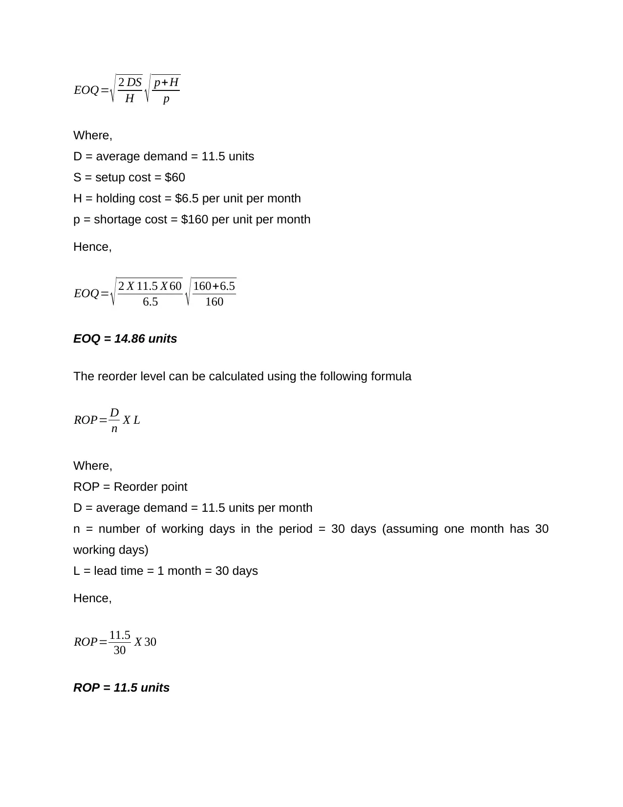
EOQ= √ 2 DS
H √ p+H
p
Where,
D = average demand = 11.5 units
S = setup cost = $60
H = holding cost = $6.5 per unit per month
p = shortage cost = $160 per unit per month
Hence,
EOQ= √ 2 X 11.5 X 60
6.5 √ 160+6.5
160
EOQ = 14.86 units
The reorder level can be calculated using the following formula
ROP= D
n X L
Where,
ROP = Reorder point
D = average demand = 11.5 units per month
n = number of working days in the period = 30 days (assuming one month has 30
working days)
L = lead time = 1 month = 30 days
Hence,
ROP=11.5
30 X 30
ROP = 11.5 units

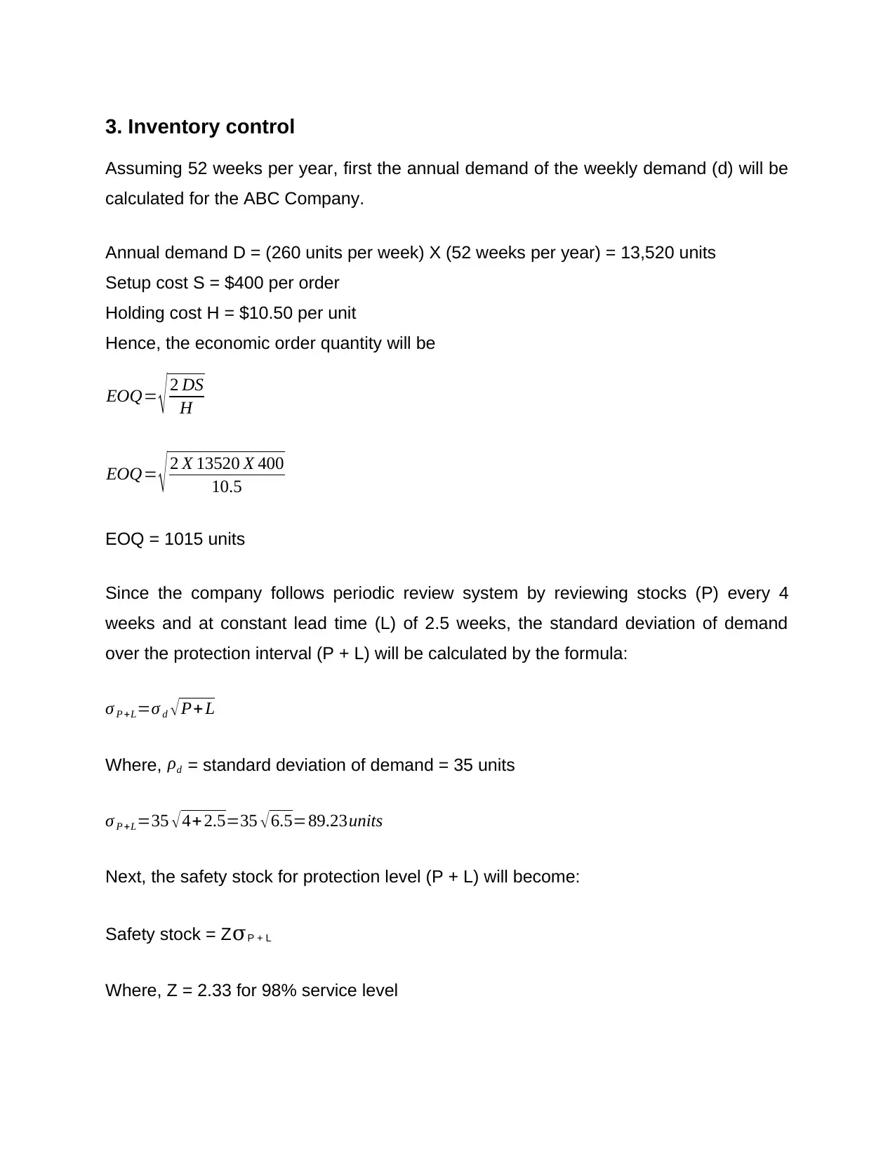
3. Inventory control
Assuming 52 weeks per year, first the annual demand of the weekly demand (d) will be
calculated for the ABC Company.
Annual demand D = (260 units per week) X (52 weeks per year) = 13,520 units
Setup cost S = $400 per order
Holding cost H = $10.50 per unit
Hence, the economic order quantity will be
EOQ= √ 2 DS
H
EOQ= √ 2 X 13520 X 400
10.5
EOQ = 1015 units
Since the company follows periodic review system by reviewing stocks (P) every 4
weeks and at constant lead time (L) of 2.5 weeks, the standard deviation of demand
over the protection interval (P + L) will be calculated by the formula:
σ P +L=σ d √ P+ L
Where, ρd = standard deviation of demand = 35 units
σ P +L=35 √ 4+ 2.5=35 √ 6.5=89.23units
Next, the safety stock for protection level (P + L) will become:
Safety stock = ZσP + L
Where, Z = 2.33 for 98% service level

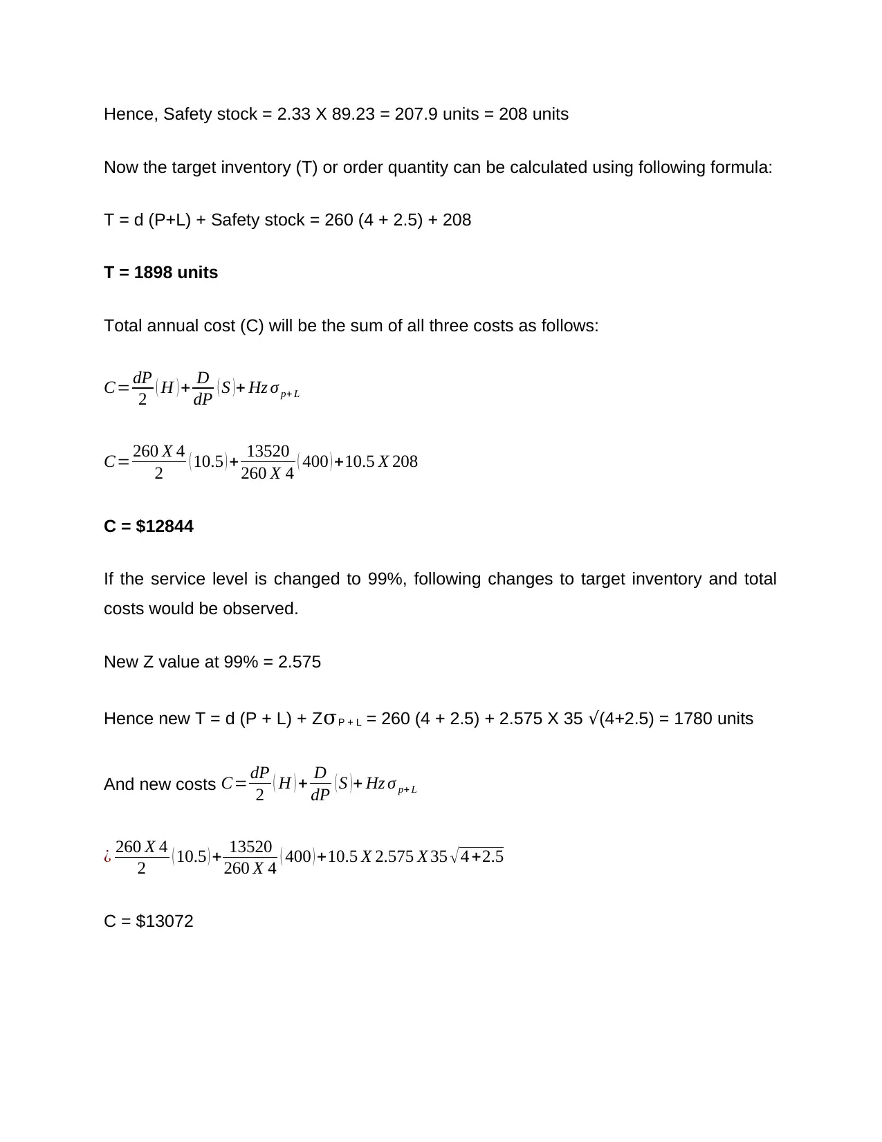
Hence, Safety stock = 2.33 X 89.23 = 207.9 units = 208 units
Now the target inventory (T) or order quantity can be calculated using following formula:
T = d (P+L) + Safety stock = 260 (4 + 2.5) + 208
T = 1898 units
Total annual cost (C) will be the sum of all three costs as follows:
C= dP
2 ( H ) + D
dP ( S )+ Hz σ p+ L
C= 260 X 4
2 ( 10.5 ) + 13520
260 X 4 ( 400 ) +10.5 X 208
C = $12844
If the service level is changed to 99%, following changes to target inventory and total
costs would be observed.
New Z value at 99% = 2.575
Hence new T = d (P + L) + ZσP + L = 260 (4 + 2.5) + 2.575 X 35 √(4+2.5) = 1780 units
And new costs C= dP
2 ( H ) + D
dP ( S )+ Hz σ p+ L
¿ 260 X 4
2 ( 10.5 ) + 13520
260 X 4 ( 400 ) +10.5 X 2.575 X 35 √ 4 +2.5
C = $13072

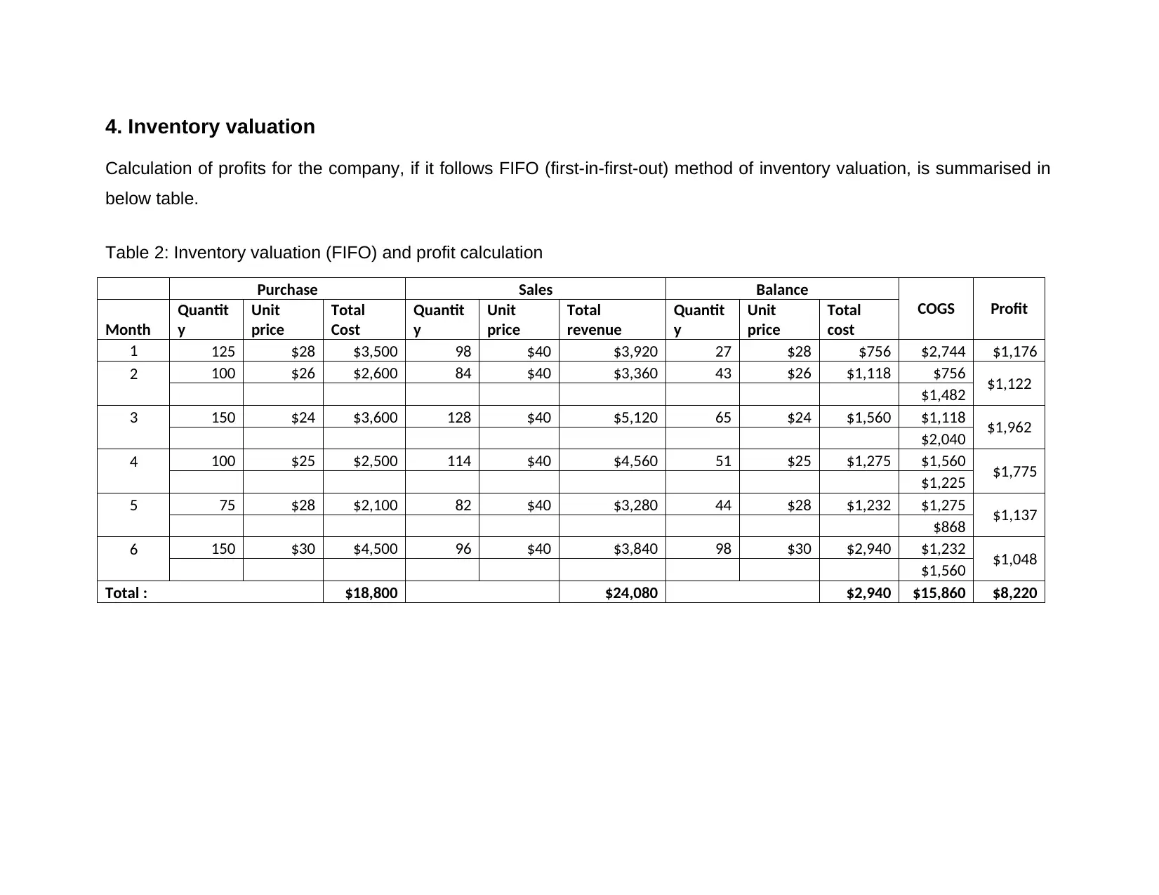
4. Inventory valuation
Calculation of profits for the company, if it follows FIFO (first-in-first-out) method of inventory valuation, is summarised in
below table.
Table 2: Inventory valuation (FIFO) and profit calculation
Purchase Sales Balance
COGS Profit
Month
Quantit
y
Unit
price
Total
Cost
Quantit
y
Unit
price
Total
revenue
Quantit
y
Unit
price
Total
cost
1 125 $28 $3,500 98 $40 $3,920 27 $28 $756 $2,744 $1,176
2 100 $26 $2,600 84 $40 $3,360 43 $26 $1,118 $756 $1,122
$1,482
3 150 $24 $3,600 128 $40 $5,120 65 $24 $1,560 $1,118 $1,962
$2,040
4 100 $25 $2,500 114 $40 $4,560 51 $25 $1,275 $1,560 $1,775
$1,225
5 75 $28 $2,100 82 $40 $3,280 44 $28 $1,232 $1,275 $1,137
$868
6 150 $30 $4,500 96 $40 $3,840 98 $30 $2,940 $1,232 $1,048
$1,560
Total : $18,800 $24,080 $2,940 $15,860 $8,220

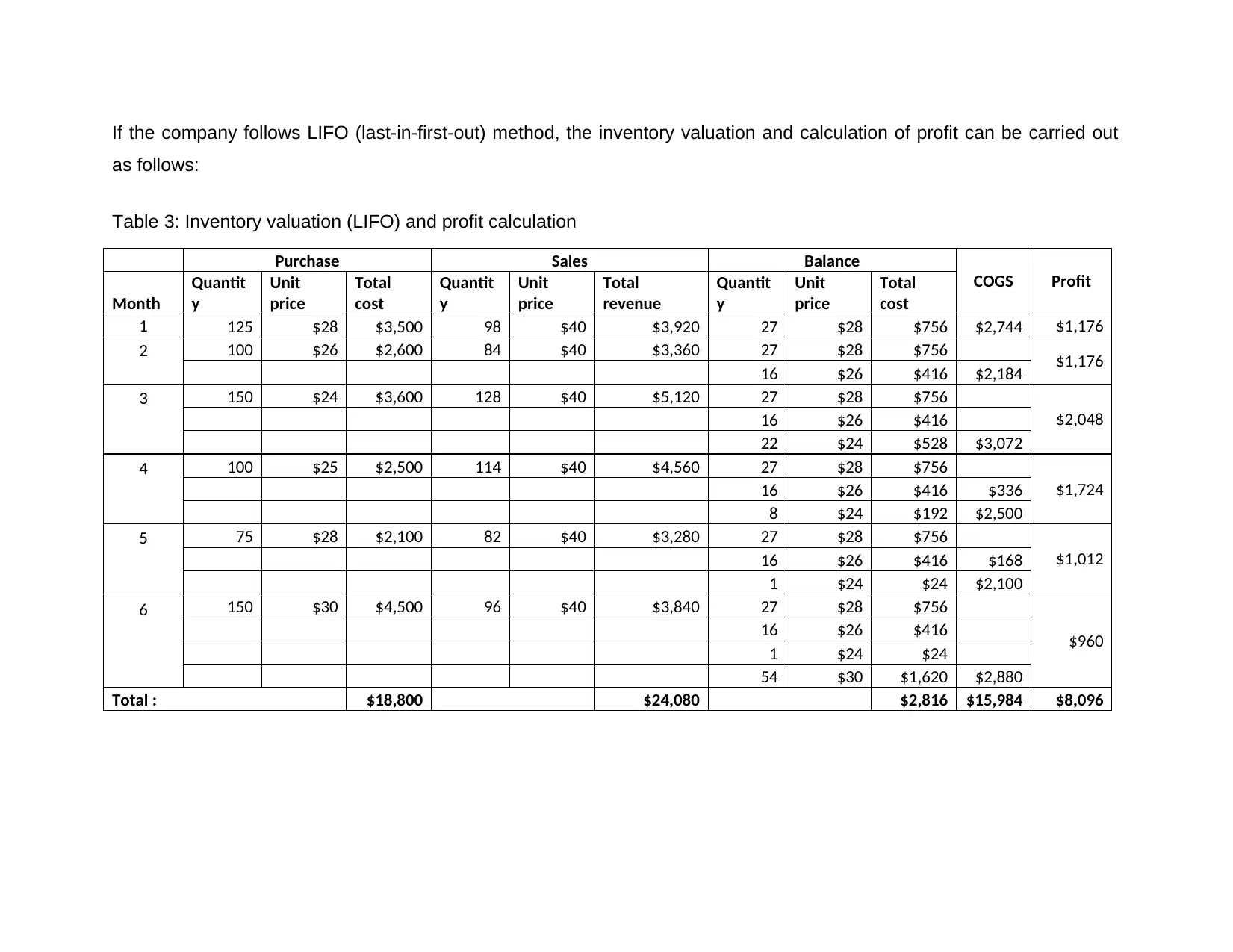
If the company follows LIFO (last-in-first-out) method, the inventory valuation and calculation of profit can be carried out
as follows:
Table 3: Inventory valuation (LIFO) and profit calculation
Purchase Sales Balance
COGS Profit
Month
Quantit
y
Unit
price
Total
cost
Quantit
y
Unit
price
Total
revenue
Quantit
y
Unit
price
Total
cost
1 125 $28 $3,500 98 $40 $3,920 27 $28 $756 $2,744 $1,176
2 100 $26 $2,600 84 $40 $3,360 27 $28 $756 $1,176
16 $26 $416 $2,184
3 150 $24 $3,600 128 $40 $5,120 27 $28 $756
$2,04816 $26 $416
22 $24 $528 $3,072
4 100 $25 $2,500 114 $40 $4,560 27 $28 $756
$1,72416 $26 $416 $336
8 $24 $192 $2,500
5 75 $28 $2,100 82 $40 $3,280 27 $28 $756
$1,01216 $26 $416 $168
1 $24 $24 $2,100
6 150 $30 $4,500 96 $40 $3,840 27 $28 $756
$960
16 $26 $416
1 $24 $24
54 $30 $1,620 $2,880
Total : $18,800 $24,080 $2,816 $15,984 $8,096

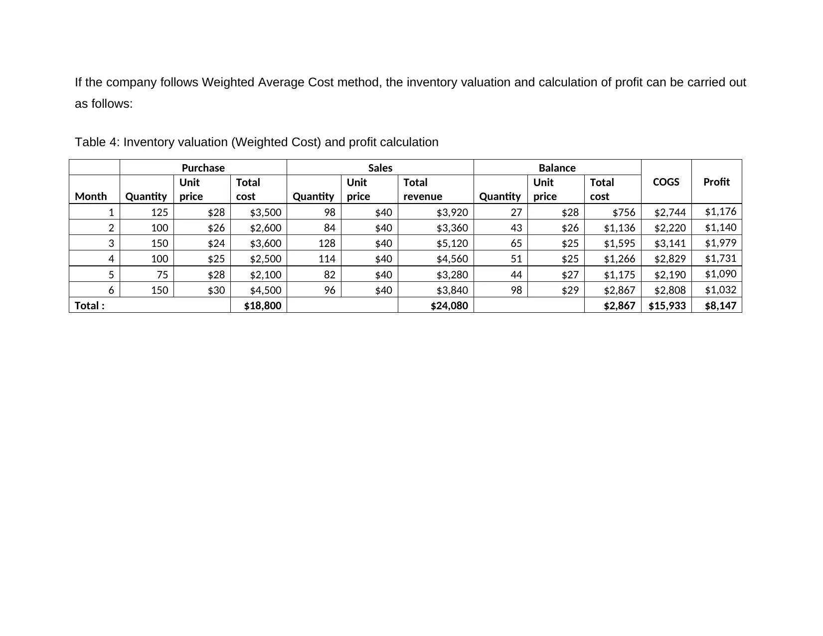
If the company follows Weighted Average Cost method, the inventory valuation and calculation of profit can be carried out
as follows:
Table 4: Inventory valuation (Weighted Cost) and profit calculation
Purchase Sales Balance
COGS Profit
Month Quantity
Unit
price
Total
cost Quantity
Unit
price
Total
revenue Quantity
Unit
price
Total
cost
1 125 $28 $3,500 98 $40 $3,920 27 $28 $756 $2,744 $1,176
2 100 $26 $2,600 84 $40 $3,360 43 $26 $1,136 $2,220 $1,140
3 150 $24 $3,600 128 $40 $5,120 65 $25 $1,595 $3,141 $1,979
4 100 $25 $2,500 114 $40 $4,560 51 $25 $1,266 $2,829 $1,731
5 75 $28 $2,100 82 $40 $3,280 44 $27 $1,175 $2,190 $1,090
6 150 $30 $4,500 96 $40 $3,840 98 $29 $2,867 $2,808 $1,032
Total : $18,800 $24,080 $2,867 $15,933 $8,147

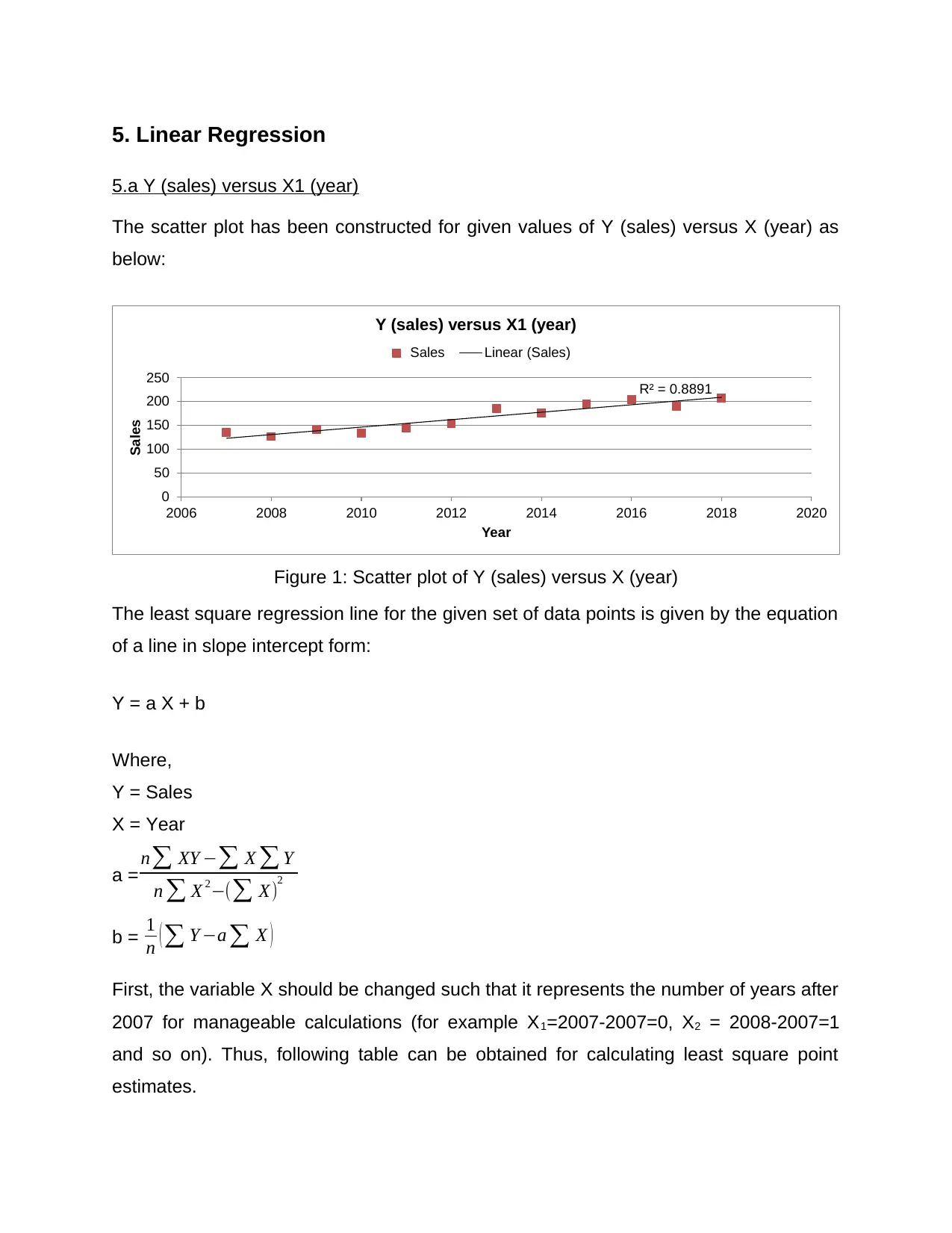
5. Linear Regression
5.a Y (sales) versus X1 (year)
The scatter plot has been constructed for given values of Y (sales) versus X (year) as
below:
R² = 0.8891
0
50
100
150
200
250
2006 2008 2010 2012 2014 2016 2018 2020
Sales
Year
Y (sales) versus X1 (year)
Sales Linear (Sales)
Figure 1: Scatter plot of Y (sales) versus X (year)
The least square regression line for the given set of data points is given by the equation
of a line in slope intercept form:
Y = a X + b
Where,
Y = Sales
X = Year
a = n∑ XY −∑ X ∑ Y
n ∑ X 2−(∑ X)2
b = 1
n (∑ Y −a ∑ X )
First, the variable X should be changed such that it represents the number of years after
2007 for manageable calculations (for example X1=2007-2007=0, X2 = 2008-2007=1
and so on). Thus, following table can be obtained for calculating least square point
estimates.

Table 5: least square point estimates for Y (sales) versus X (year)
X Y XY X2 Y2
0 136 0 0 18496
1 127 127 1 16129
2 141 282 4 19881
3 134 402 9 17956
4 145 580 16 21025
5 154 770 25 23716
6 186 1116 36 34596
7 176 1232 49 30976
8 195 1560 64 38025
9 204 1836 81 41616
10 190 1900 100 36100
11 208 2288 121 43264
ΣX = 66 ΣY = 1996 ΣXY = 12093 ΣX2 = 506 ΣY2 = 341780
Now, a = n∑ XY −∑ X ∑ Y
n ∑ X 2−(∑ X)2
a = ( 12 X 12093 ) −(66 X 1996)
(12 X 506)−(66)2
a = 7.8
and b = 1
n ( ∑ Y −a ∑ X )
b = 1
12 ( 1996−7.8 X 66 )
b = 123.45
Hence, the future sales can be forecasted by the following formula
Y = 7.8 X + 123.45
Finally, the correlation coefficient is calculated using the formula: