25503 Investment Analysis Assignment - Part I Summer 2018 - University

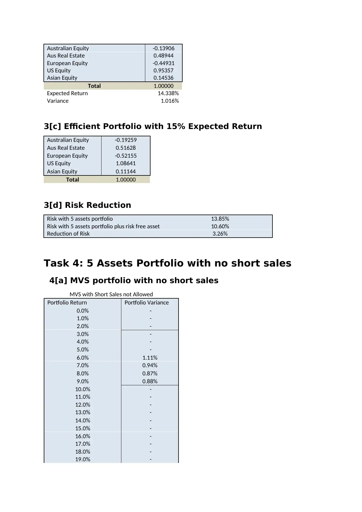
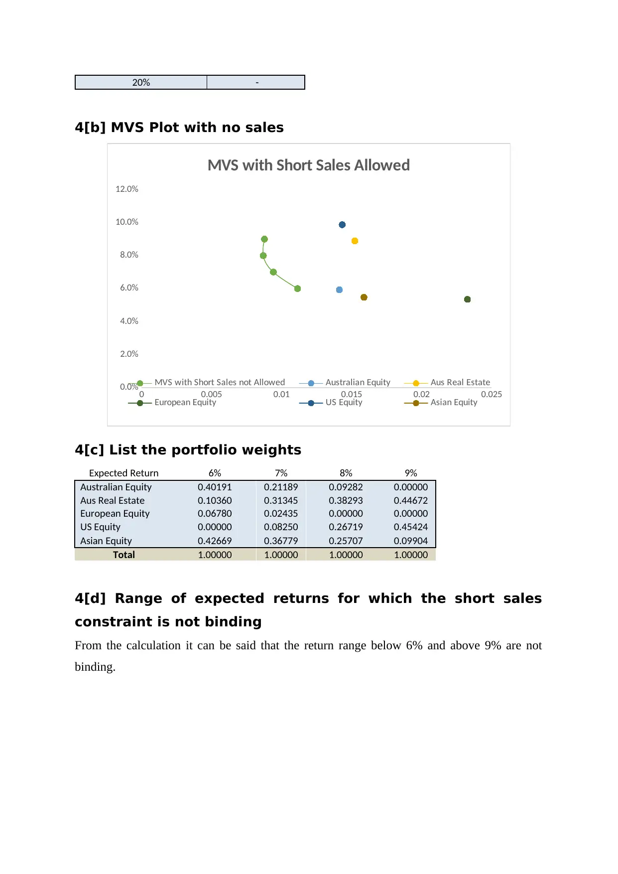
This assignment presents a detailed investment analysis, focusing on portfolio construction and risk management. It begins with a five-asset portfolio, exploring weekly returns, mean-variance analysis, efficient and inefficient assets, and the calculation of key parameters like A, B, C, and delta. The analysis includes MVS plots with and without short sales, determination of the global minimum variance portfolio, and efficient portfolio weights for a 15% expected return. The second part of the assignment expands the portfolio to include a commodity (Silver), repeating the analysis and assessing the impact on risk and return. The final sections incorporate a risk-free rate, construct a tangency portfolio, and analyze portfolio performance with and without short-selling constraints. The assignment demonstrates the application of financial modeling techniques to optimize investment strategies and manage portfolio risk.

25503 Investment Analysis
Assignment - Part I
Summer 2018
Name of the Student
Name of the University

Task 1: Portfolio with 5 asset classes [when short
sells allowed]
1[a] Simple weekly return
In order to convert index values into weekly return, the below mentioned excel function is
used:
This return values have been used later on to perform further analysis.
1[b] Vector of Means and Variance Covariance Matrix
The first step of analysis is calculating annualised return of individual stocks and variance
covariance matrix. While calculating annualised return, the analyst first identified the average
return of all 5 assets over the 357 weeks period using the excel average formula
‘=AVERAGE(G4:G360) [for Australian Equity] and then multiplied the value by 52 to get
annualised return. The below table is showing the annualised return of all 5 assets:
Now to find out the vector of return, excel transpose array function
‘{=TRANSPOSE(C2:G3)} is used. The vector of return is as mentioned below:
The annualised variance and covariance is calculated using excel covariance function and the
matrix is as followed:

1[c] Efficient and inefficient assets:
The return matrix is showing the fact that US equity is the most dominant one among the five
assets. In other words, US equity is the efficient asset followed by Australian real estate. On
the other hand, European Equity, Australian Equity, and Asian Equity can be considered as
inefficient asset classes for this specific case.
Now, if Australian equity and Australian real estate are taken into comparison, then it can be
said that Australian real estate dominates Australian equity. Similarly, Australian real estate
dominates European equity. Again, US equity dominates all other 4 assets.
1[d] Values of A, B, C and ∆
In order to calculate A, B, C and ∆, the following excel functions are used:
A = {=MMULT(TRANSPOSE(D7:D11),MMULT(MINVERSE(C15:G19),C7:C11))}
B = {=MMULT(TRANSPOSE(C7:C11),MMULT(MINVERSE(C15:G19),C7:C11))}
C = {=MMULT(TRANSPOSE(D7:D11),MMULT(MINVERSE(C15:G19),D7:D11))}
And ∆ = BC – A^2

1[e] MVS plot with short sales allowed with expected return
0% to 20%
0.50% 1.00% 1.50% 2.00% 2.50% 3.00% 3.50% 4.00% 4.50% 5.00%
0%
5%
10%
15%
20%
25%
MVS with Short Sales Allowed
MVS with Short Sales Allowed Australian Equity Aus Real Estate European Equity
US Equity Asian Equity
1[f] Global Minimum Variance Portfolio [MVP]
The global minimum variance portfolio is the main proficient stock portfolio whose weights
don't rely upon the normal returns. Along the efficient frontier line, one can stay away from

extraordinary estimation chance by putting into this portfolio. By and by, there remains an
impressive estimation chance concerning the covariance grid. Excel solver is used to find out
the global minimum variance portfolio and below is the details of MVP for this case:
Australian Equity -0.43527
Aus Real Estate 0.63797
European Equity -0.84909
US Equity 1.68876
Asian Equity -0.04237
Total 1.00000
Expected Return 8.865%
Variance 0.841%
1[g] Portfolio weights for the efficient portfolio with 15%
expected return
Australian Equity -0.43527
Aus Real Estate 0.63797
European Equity -0.84909
US Equity 1.68876
Asian Equity -0.04237
Total 1.00000
Task 2: Portfolio with 5 assets and one
commodity
2[a] Adding one commodity in portfolio
In the previous section a 5 assets portfolio has been created and the portfolio return as well as
risk has been reported. Now, as per management wish, in order to involve one commodity,
the analyst needs to check return of all three commodities as well as their association with
existing 5 asset classes. The first step was performing a correlation analysis as the aim was to
find out which commodity is less correlated with rest asset classes. This helped the analyst to
diversify the risk of the portfolio.

Now from the above correlation table, it can be said that Silver is comparatively less
correlated with existing 5 assets. Thus the further analysis has been performed with
considering Silver as the 6th asset in the existing 5 assets portfolio.
2[b] Vector of return and Variance-Covariance Matrix
The above mentioned process is repeated once again considering 5 existing assets and Silver
to find the return vector and variance co-variance matrix. Below is the details:
Vector of Return
Australian Equity 0.059276544
Aus Real Estate 0.088916323
European Equity 0.053460472
US Equity 0.098762159
Asian Equity 0.054699653
Silver -0.072817533
Variance
Covariance Matrix
Australian
Equity
Aus Real
Estate
European
Equity US Equity Asian Equity Silver
Australian Equity 0.014116466 0.008471434 0.010208357 0.007727624 0.009371441 0.003001975
Aus Real Estate 0.008471434 0.015227039 0.003710392 0.003403274 0.003959206 0.000450125
European Equity 0.010208357 0.003710392 0.023269588 0.014599615 0.014119352 0.009776121
US Equity 0.007727624 0.003403274 0.014599615 0.014326396 0.00986241 0.005681009
Asian Equity 0.009371441 0.003959206 0.014119352 0.00986241 0.015877967 0.006774735
Silver 0.003001975 0.000450125 0.009776121 0.005681009 0.006774735 0.056531949
2[c] Values of A, B, C and ∆
In order to calculate A, B, C and ∆, the following excel functions are used:
A = {=MMULT(TRANSPOSE(E18:E23),MMULT(MINVERSE(C27:H32),C18:C23))}
B = {=MMULT(TRANSPOSE(C7:C11),MMULT(MINVERSE(C15:G19),C7:C11))}
C = {=MMULT(TRANSPOSE(D7:D11),MMULT(MINVERSE(C15:G19),D7:D11))}
And ∆ = BC – A^2
A 9.467454351

B 1.430902389
C 126.7417072
∆ 91.72231975
2[d] MVS plot with short sales allowed with expected return
-10% to 30%
MVS with Short Sales Allowed 2
Portfolio Return
Portfolio
Variance
-10% 0.0500620
82
-7% 0.0368217
94
-4% 0.0260687
42
-1% 0.0178029
25
2% 0.0120243
45
5% 0.0087330
02
8% 0.0079288
95
11% 0.0096120
23
14% 0.0137823
88
17% 0.0204399
89
20% 0.0295848
27
23% 0.0412169
86
26% 0.0553362
1
29% 0.0719427
55
30% 0.0780317
67

0.005 0.01 0.015 0.02 0.025 0.03 0.035 0.04 0.045 0.05
0%
5%
10%
15%
20%
25%
MVS with Short Sales Allowed 2
MVS with Short Sales Allowed 2 Australian Equity Aus Real Estate
European Equity US Equity Asian Equity
MVS with Short Sales Allowed
The above figure is showing both MVS plot with 5 assets as well as MVS plot with 6 assets.
It can be infer that the addition of Silver helped the analyst to diversify the risk level.
2[e] New portfolio weights for the efficient portfolio with
15% expected return
Efficient Portfolio with 15% Expected Return
Australian Equity -0.195220
Aus Real Estate 0.577629
European Equity -0.463966
US Equity 1.246786
Asian Equity -0.001190
Silver -0.164039
Total 1.000000
2[f] Risk Reduction
The risk of an individual stock can be estimated by the variance on individual asset class. The
risk of individual stock can be diminished through diversification. Diversification decreases
the fluctuation when the costs of individual resources are not splendidly associated. As it
were, speculators can lessen their introduction to singular resources by holding a diversified
portfolio of stocks. Accordingly, diversification will take into consideration a similar
portfolio come back with decreased hazard. The below table is showing that addition of
Silver commodity reduces the risk by 1.25%.
Risk with 5 assets portfolio 0.138546745

Risk with 6 assets portfolio 0.126005727
Reduction of Risk 0.012541018
Task 3: Mean Variance Portfolio with risk free
rate
3[a] MVS Plot with risk free rate
MVS with Short Sales Allowed
Portfolio Return Portfolio Variance
0% 4.88%
2% 3.63%
4% 2.61%
6% 1.83%
8% 1.27%
10% 0.94%
12% 0.84%
14% 0.97%
16% 1.33%
18% 1.92%
20% 2.74%
22% 3.78%
24% 5.06%
26% 6.57%
0.00% 1.00% 2.00% 3.00% 4.00% 5.00% 6.00% 7.00%
0%
5%
10%
15%
20%
25%
30%
MVS with Short Sales Allowed
MVS with Short Sales Allowed Tangency Portfolio
3[b] Tangency Portfolio
Tangency Portfolio

Australian Equity -0.13906
Aus Real Estate 0.48944
European Equity -0.44931
US Equity 0.95357
Asian Equity 0.14536
Total 1.00000
Expected Return 14.338%
Variance 1.016%
3[c] Efficient Portfolio with 15% Expected Return
Australian Equity -0.19259
Aus Real Estate 0.51628
European Equity -0.52155
US Equity 1.08641
Asian Equity 0.11144
Total 1.00000
3[d] Risk Reduction
Risk with 5 assets portfolio 13.85%
Risk with 5 assets portfolio plus risk free asset 10.60%
Reduction of Risk 3.26%
Task 4: 5 Assets Portfolio with no short sales
4[a] MVS portfolio with no short sales
MVS with Short Sales not Allowed
Portfolio Return Portfolio Variance
0.0% -
1.0% -
2.0% -
3.0% -
4.0% -
5.0% -
6.0% 1.11%
7.0% 0.94%
8.0% 0.87%
9.0% 0.88%
10.0% -
11.0% -
12.0% -
13.0% -
14.0% -
15.0% -
16.0% -
17.0% -
18.0% -
19.0% -

20% -
4[b] MVS Plot with no sales
0 0.005 0.01 0.015 0.02 0.025
0.0%
2.0%
4.0%
6.0%
8.0%
10.0%
12.0%
MVS with Short Sales Allowed
MVS with Short Sales not Allowed Australian Equity Aus Real Estate
European Equity US Equity Asian Equity
4[c] List the portfolio weights
Expected Return 6% 7% 8% 9%
Australian Equity 0.40191 0.21189 0.09282 0.00000
Aus Real Estate 0.10360 0.31345 0.38293 0.44672
European Equity 0.06780 0.02435 0.00000 0.00000
US Equity 0.00000 0.08250 0.26719 0.45424
Asian Equity 0.42669 0.36779 0.25707 0.09904
Total 1.00000 1.00000 1.00000 1.00000
4[d] Range of expected returns for which the short sales
constraint is not binding
From the calculation it can be said that the return range below 6% and above 9% are not
binding.