MIS775: Investment Portfolio Optimisation with Decision Models

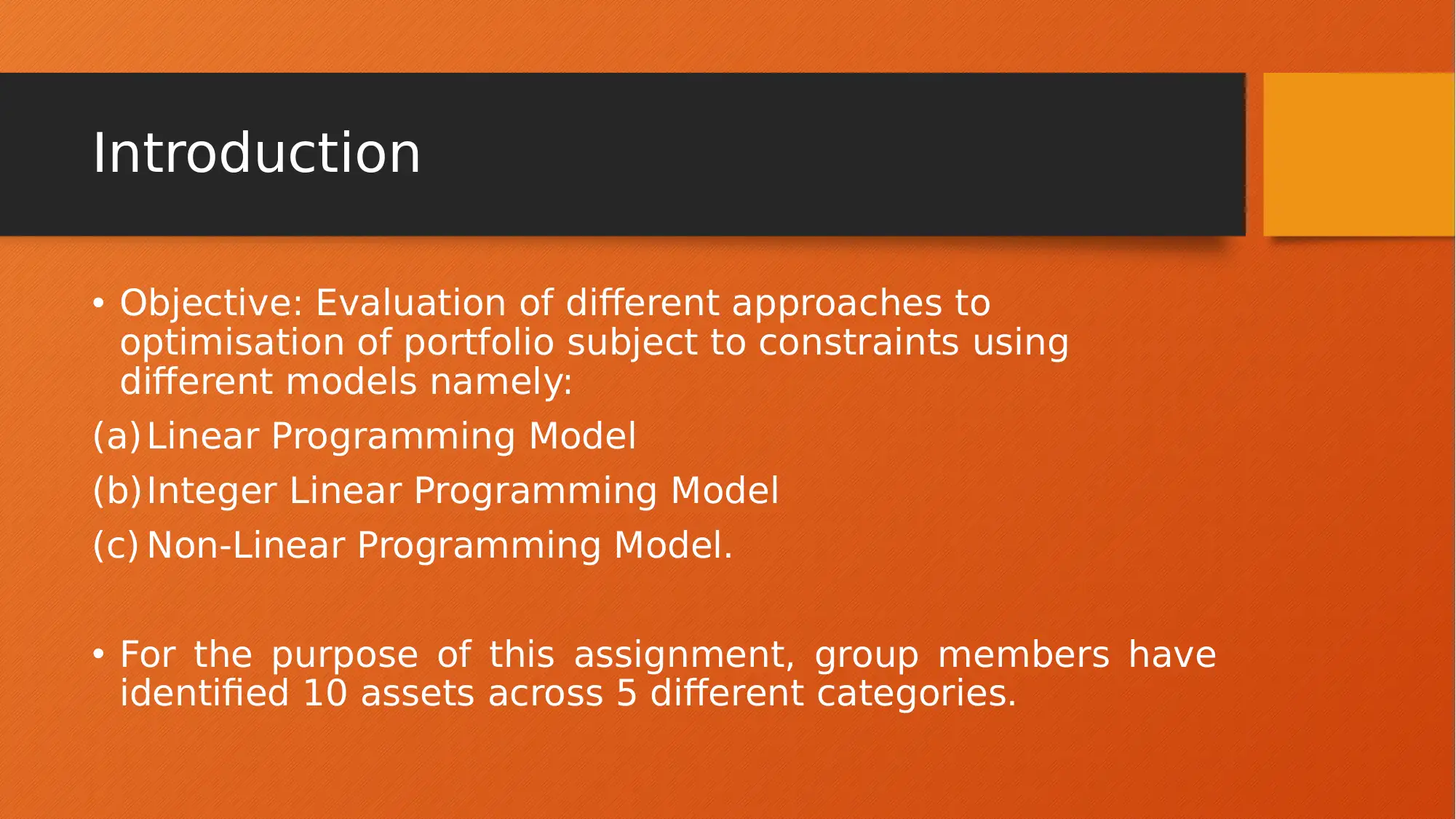
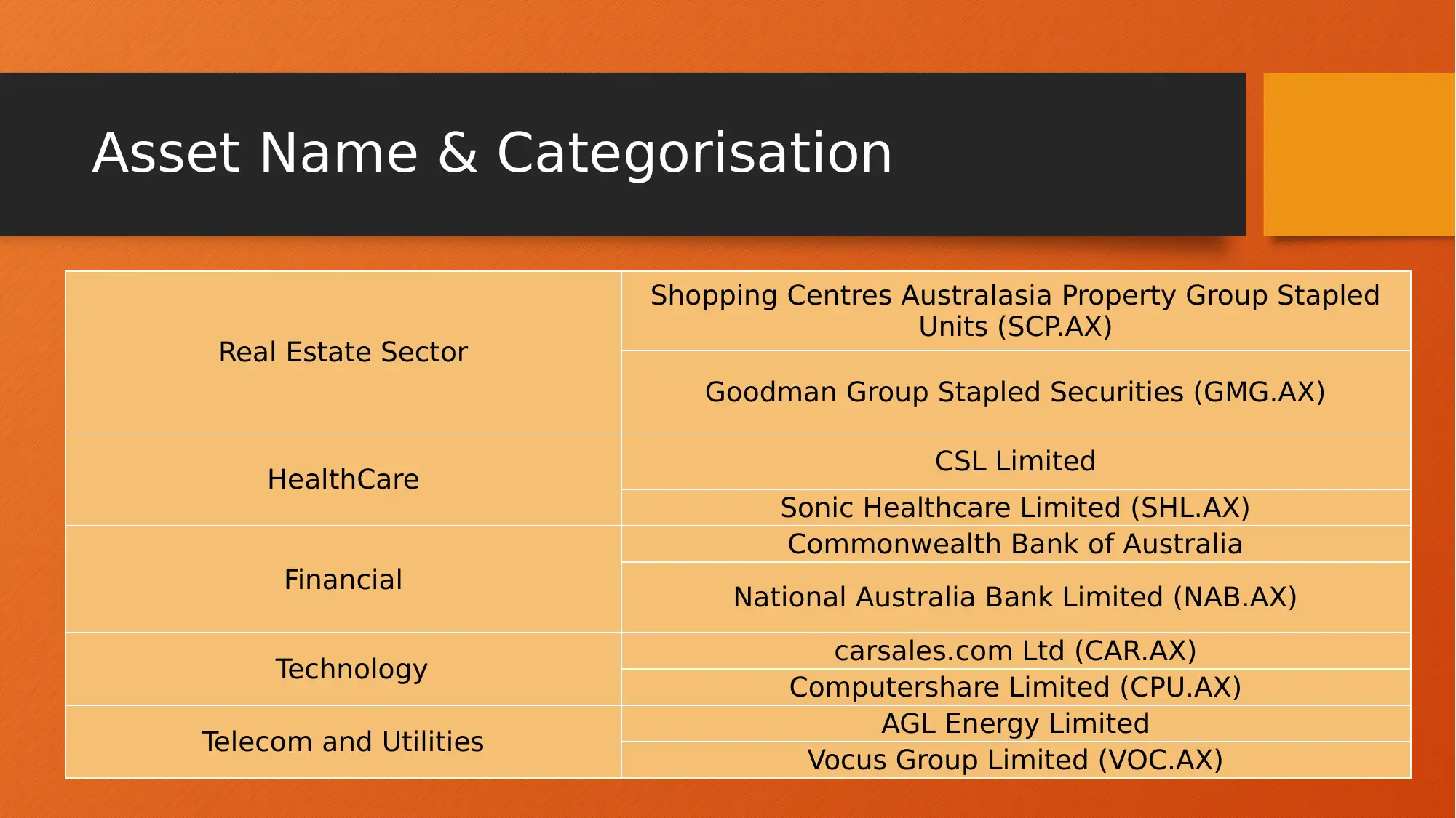
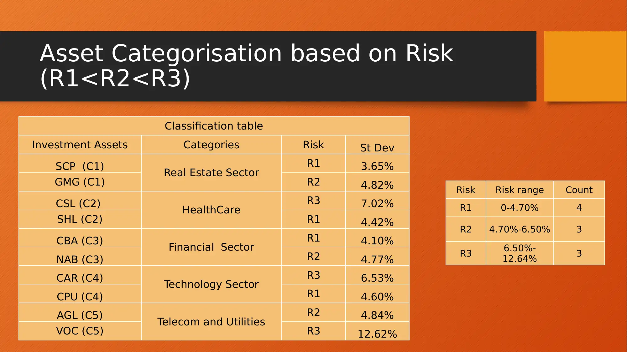
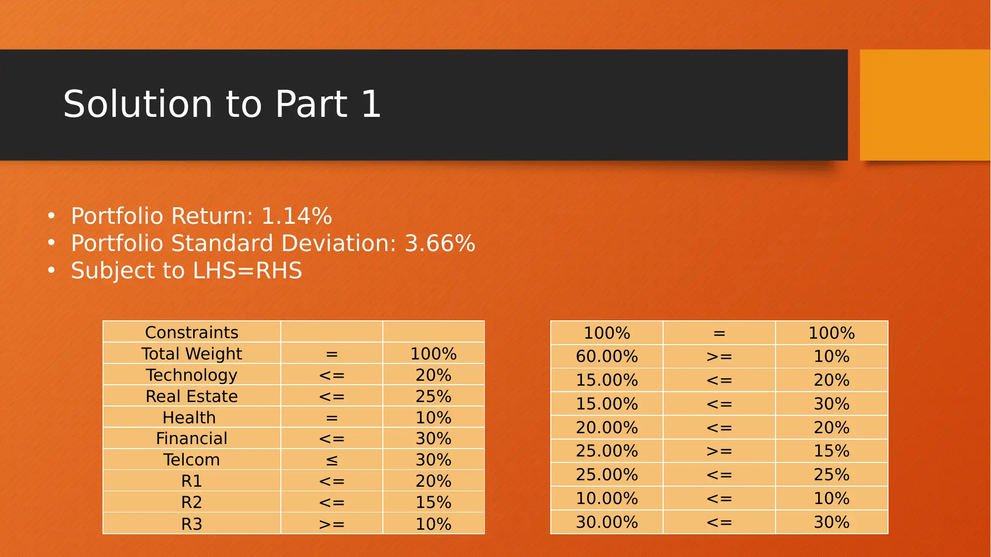
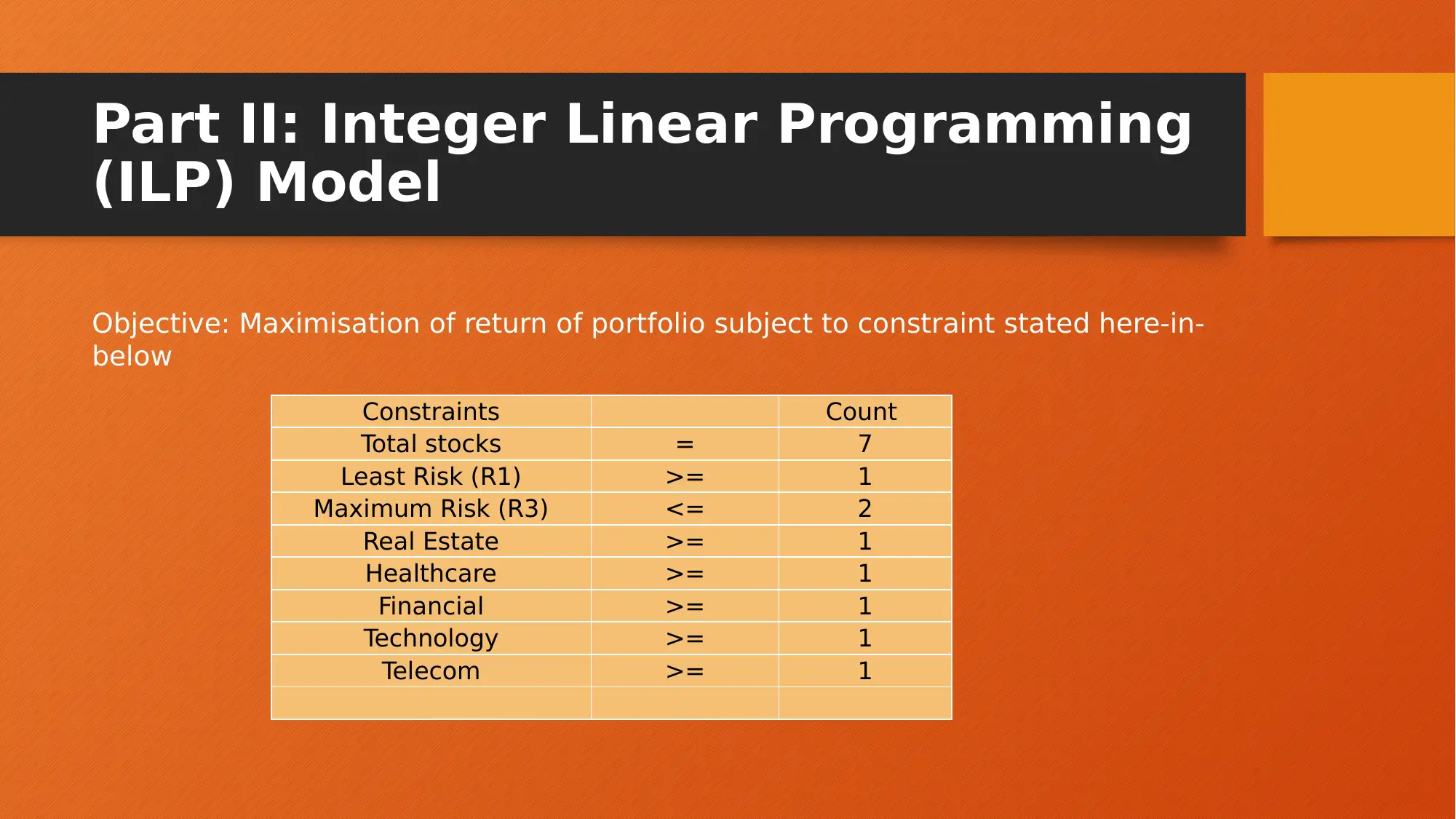
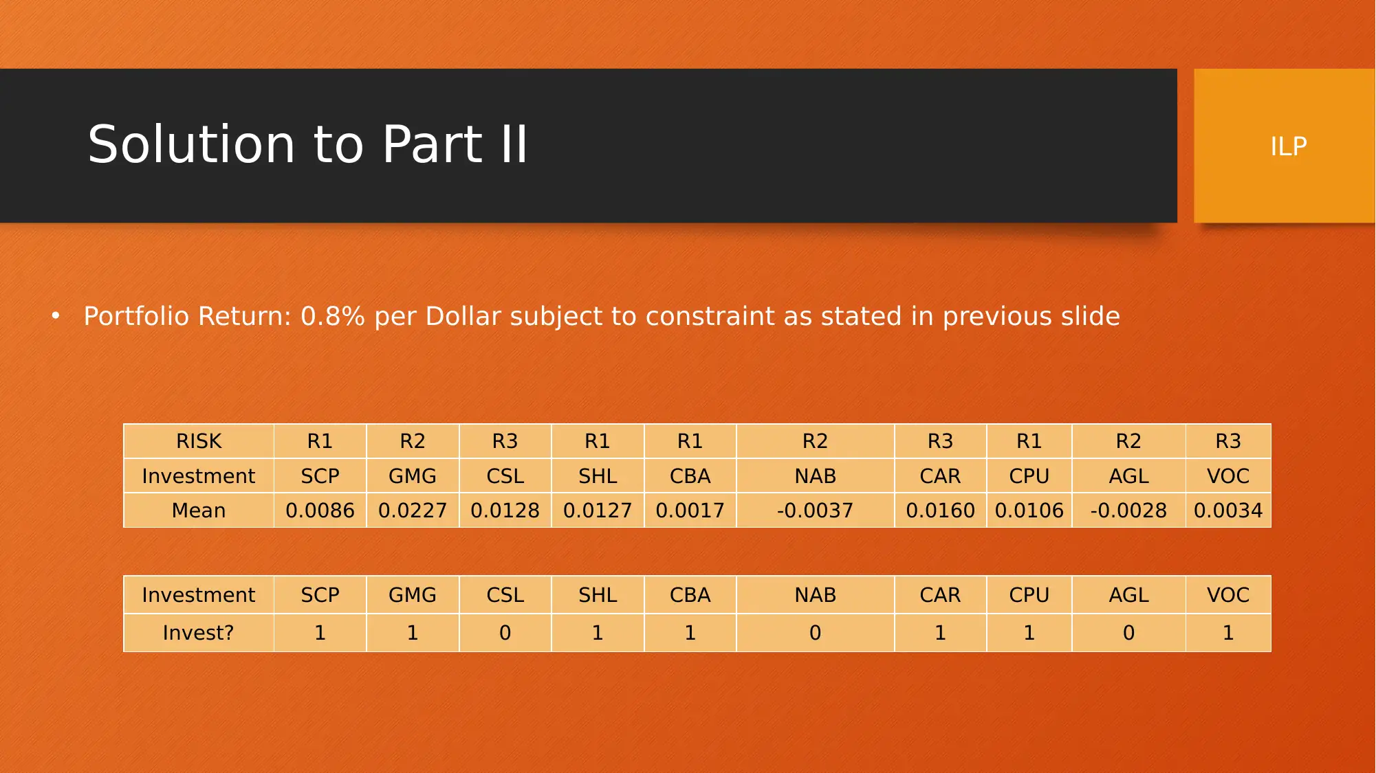
This project report presents an analysis of investment portfolio optimisation using three different modelling approaches: Linear Programming (LP), Integer Linear Programming (ILP), and Non-Linear Programming (NLP). The analysis is conducted using financial data of 10 assets across five different categories, with data collected over a period of 37 months, and the objective is to maximize portfolio return. The report details the formulation of each model, including objective functions and constraints, and presents the results obtained from each model, including portfolio returns, standard deviations, and asset weights. The LP model provides insights through sensitivity analysis. The NLP model explores different objectives, such as maximizing return with risk constraints and maximizing utility with various risk aversion parameters (r). The report concludes with a comparison of the models, highlighting the NLP B model as the most optimized portfolio, offering the highest return for a given risk level and recommending a strategy of fixed return with minimum risk.

Decision Modelling for Business
Analytics
Investment Portfolio Optimisation
Group No:

Introduction
• Objective: Evaluation of different approaches to
optimisation of portfolio subject to constraints using
different models namely:
(a) Linear Programming Model
(b)Integer Linear Programming Model
(c) Non-Linear Programming Model.
• For the purpose of this assignment, group members have
identified 10 assets across 5 different categories.

Asset Name & Categorisation
Real Estate Sector
Shopping Centres Australasia Property Group Stapled
Units (SCP.AX)
Goodman Group Stapled Securities (GMG.AX)
HealthCare CSL Limited
Sonic Healthcare Limited (SHL.AX)
Financial
Commonwealth Bank of Australia
National Australia Bank Limited (NAB.AX)
Technology carsales.com Ltd (CAR.AX)
Computershare Limited (CPU.AX)
Telecom and Utilities AGL Energy Limited
Vocus Group Limited (VOC.AX)

Asset Categorisation based on Risk
(R1<R2<R3)
Classification table
Investment Assets Categories Risk St Dev
SCP (C1) Real Estate Sector R1 3.65%
GMG (C1) R2 4.82%
CSL (C2) HealthCare R3 7.02%
SHL (C2) R1 4.42%
CBA (C3) Financial Sector R1 4.10%
NAB (C3) R2 4.77%
CAR (C4) Technology Sector R3 6.53%
CPU (C4) R1 4.60%
AGL (C5) Telecom and Utilities R2 4.84%
VOC (C5) R3 12.62%
Risk Risk range Count
R1 0-4.70% 4
R2 4.70%-6.50% 3
R3 6.50%-
12.64% 3

Data Formulation
• The financial stock values for each of these 10 assets were collected over a period of 37
months
• Using this data we calculated the following:
(a) Average and monthly returns for each stock
(b) Average and monthly risk associated with each stock
(c) Average annual return for each stock
• In addition to this, all assets chosen satisfy the following general constraints:
(a) 37 months of data should be collected for each of these assets up to and including
Feb 2020.
(b) The assets should be selected from 5 different categories and there should 2 assets
in each category.
(c)These assets must span a reasonable range of risks and must be classified into 3 risk
groups (R1, R2, R3), with R1 being the least volatile and R4 being the most volatile.
(d) Each risk group must contains at least 3 assets.

Part 1: Linear Programming(LP)-
Objective & Constraint
Constraints
Total Weight = 100%
Technology <= 20%
Real Estate <= 25%
Health = 10%
Financial <= 30%
Telcom ≤ 30%
R1 <= 20%
R2 <= 15%
R3 >= 10%
Objective: Maximisation of return of portfolio subject to constraint stated
here-in-below

Solution to Part 1
• Portfolio Return: 1.14%
• Portfolio Standard Deviation: 3.66%
• Subject to LHS=RHS
100% = 100%
60.00% >= 10%
15.00% <= 20%
15.00% <= 30%
20.00% <= 20%
25.00% >= 15%
25.00% <= 25%
10.00% <= 10%
30.00% <= 30%
Constraints
Total Weight = 100%
Technology <= 20%
Real Estate <= 25%
Health = 10%
Financial <= 30%
Telcom ≤ 30%
R1 <= 20%
R2 <= 15%
R3 >= 10%

Contd:
SCP GMG CSL SHL CBA NAB CAR CPU AGL VOC
Investment weights 0.00% 25.00
% 10.00% 0.00% 15.00% 0.00% 20.00
% 0.00% 0.00% 30.00
%
LP

Interpretation of Sensitivity Analysis
Final Reduced Objective Allowable Allowable
Cell Name Valu
e Cost Coefficient Increase Decrease
$D$2
2
Investment weights
SCP 0
-
0.0140152
73
0.0086436
08
0.0140152
73 1E+30
$E$2
2
Investment weights
GMG 0.25 0 0.0226588
81 1E+30 0.0140152
73
$F$2
2
Investment weights
CSL 0.1 0 0.0127884
69 1E+30 0.0001041
33
$G$2
2
Investment weights
SHL 0
-
0.0001041
33
0.0126843
36
0.0001041
33 1E+30
$H$2
2
Investment weights
CBA 0.15 0 0.0016842
92
0.0017106
89
0.0054025
12
$I$22 Investment weights
NAB 0
-
0.0054025
12
-
0.0037182
2
0.0054025
12 1E+30
$J$22 Investment weights
CAR 0.2 0 0.0159711
77 1E+30 0.0053925
16
$K$2
2
Investment weights
CPU 0
-
0.0053925
16
0.0105786
61
0.0053925
16 1E+30
$L$2
2
Investment weights
AGL 0
-
0.0062155
15
-
0.0028205
34
0.0062155
15 1E+30
Final Shadow Constraint Allowable Allowable
Cell Name Valu
e Price R.H. Side Increase Decrease
$B$6
1 LHS 1 0.0016842
92 1 0.05 0.15
$B$6
3 LHS 0.6 0 0.1 0.5 1E+30
$B$6
4 LHS 0.15 0 0.2 1E+30 0.05
$B$6
5 LHS 0.15 0 0.3 1E+30 0.15
$B$6
6 LHS 0.2 0.0142868
85 0.2 0.15 0.05
$B$6
7 LHS 0.25 0 0.15 0.1 1E+30
$B$6
8 LHS 0.25 0.0209745
88 0.25 0.15 0.05
$B$6
9 LHS 0.1 0.0111041
77 0.1 0.15 0.05
$B$7
0 LHS 0.3 0.0017106
89 0.3 0.15 0.05

Interpretation of Sensitivity Analysis
• On perusal of the above tables, it may be inferred that the there is allowable increase
for five assets in the portfolio and allowable decrease of five asset in the portfolio.
• Further, the reduction in each of the asset has been duly shown to achieve the desired
portfolio.
• Probable increase or decrease in constraint which can impact the return of the portfolio
like allowable increase for weights is 0.05 (increase) to 0.15 (decrease)
• Similarly, Investment in R3 cannot be exceeded further.
• For R2 it has been stated that allowable increase of 0.5 is permitted and so on.

Part II: Integer Linear Programming
(ILP) Model
Objective: Maximisation of return of portfolio subject to constraint stated here-in-
below
Constraints Count
Total stocks = 7
Least Risk (R1) >= 1
Maximum Risk (R3) <= 2
Real Estate >= 1
Healthcare >= 1
Financial >= 1
Technology >= 1
Telecom >= 1

Solution to Part II
• Portfolio Return: 0.8% per Dollar subject to constraint as stated in previous slide
RISK R1 R2 R3 R1 R1 R2 R3 R1 R2 R3
Investment SCP GMG CSL SHL CBA NAB CAR CPU AGL VOC
Mean 0.0086 0.0227 0.0128 0.0127 0.0017 -0.0037 0.0160 0.0106 -0.0028 0.0034
Investment SCP GMG CSL SHL CBA NAB CAR CPU AGL VOC
Invest? 1 1 0 1 1 0 1 1 0 1
ILP