ABB IRB140 Robot: DH Parameter Table and Kinematics Analysis

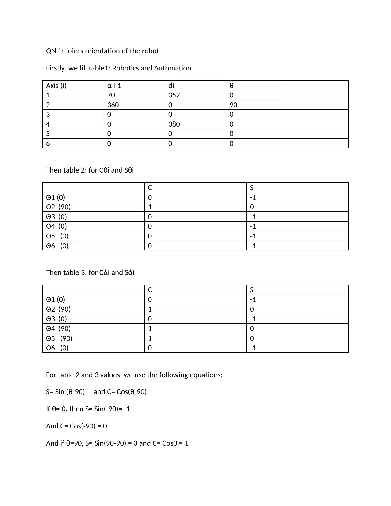
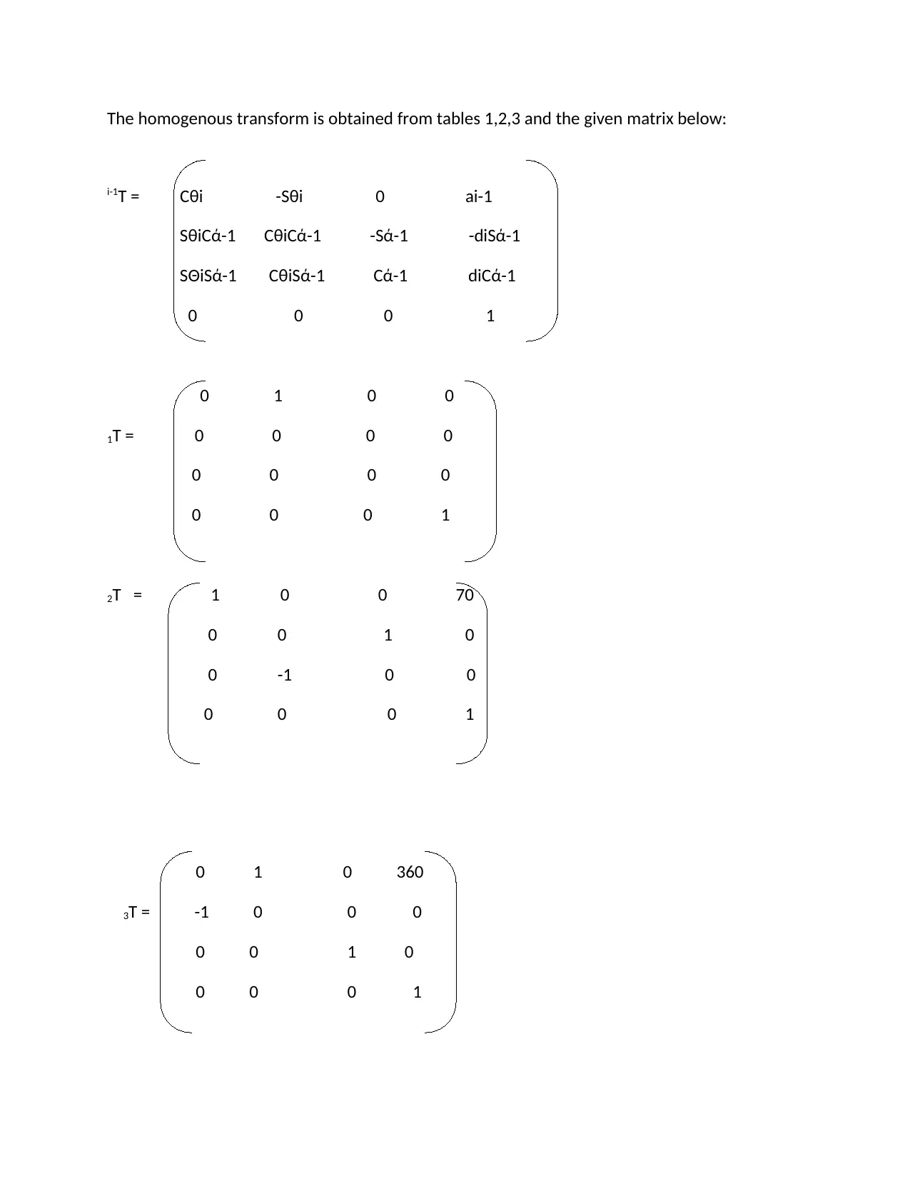
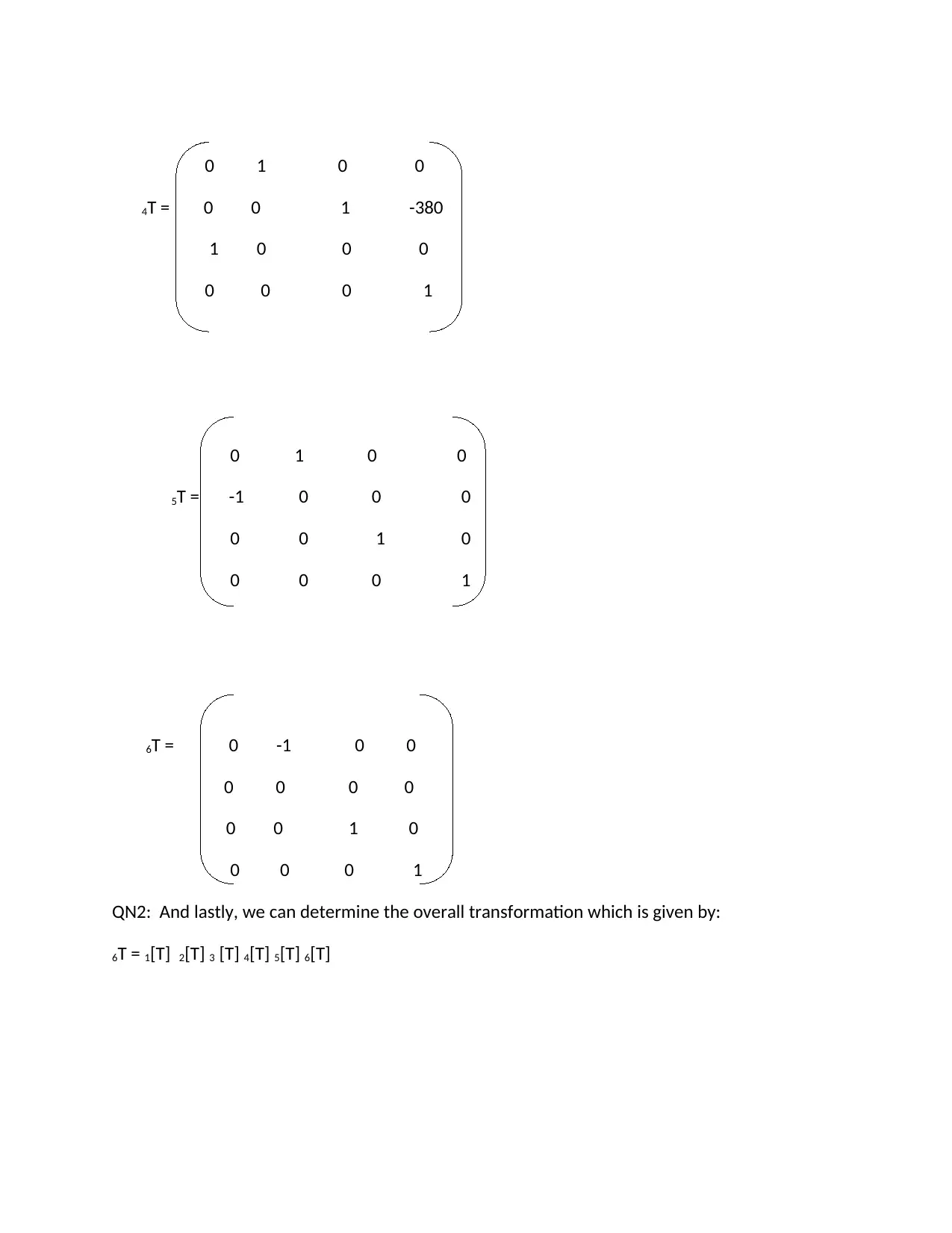
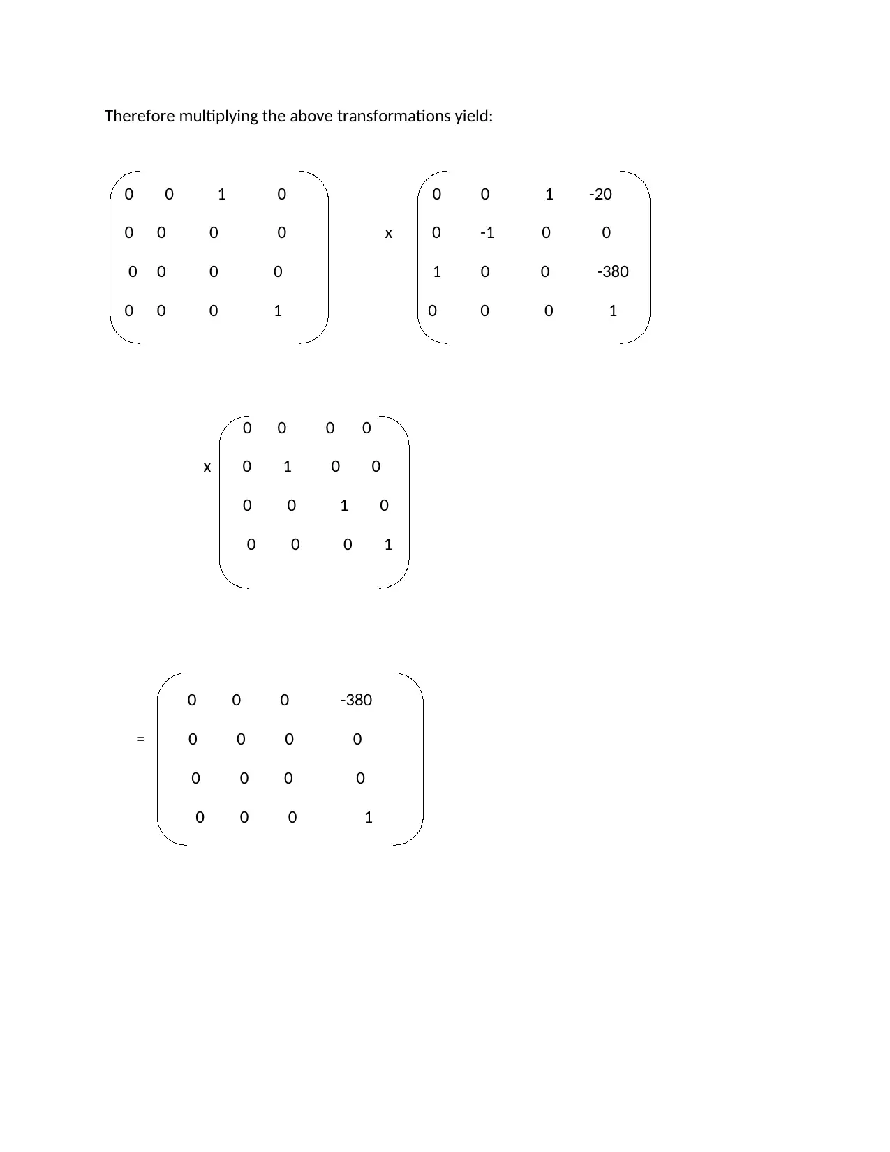
This project analyzes the kinematics of the ABB IRB140 robot, a common industrial manipulator. The solution begins by constructing a Denavit-Hartenberg (DH) parameter table to define the robot's link and joint characteristics, including axis orientations and offsets. Using the DH parameters, the individual transformation matrices for each link are derived. These matrices are then multiplied to obtain the overall homogeneous transformation matrix, which describes the position and orientation of the robot's end-effector relative to its base. The solution includes the calculation of the transformation matrices and the final overall transformation matrix. The forward kinematics solution yields the position and orientation of the robot's end-effector based on the joint angles.

QN 1: Joints orientation of the robot
Firstly, we fill table1: Robotics and Automation
Axis (i) α i-1 di θ
1 70 352 0
2 360 0 90
3 0 0 0
4 0 380 0
5 0 0 0
6 0 0 0
Then table 2: for Cθi and Sθi
C S
Θ1 (0) 0 -1
Θ2 (90) 1 0
Θ3 (0) 0 -1
Θ4 (0) 0 -1
Θ5 (0) 0 -1
Θ6 (0) 0 -1
Then table 3: for Cάi and Sάi
C S
Θ1 (0) 0 -1
Θ2 (90) 1 0
Θ3 (0) 0 -1
Θ4 (90) 1 0
Θ5 (90) 1 0
Θ6 (0) 0 -1
For table 2 and 3 values, we use the following equations:
S= Sin (θ-90) and C= Cos(θ-90)
If θ= 0, then S= Sin(-90)= -1
And C= Cos(-90) = 0
And if θ=90, S= Sin(90-90) = 0 and C= Cos0 = 1

The homogenous transform is obtained from tables 1,2,3 and the given matrix below:
i-1T = Cθi -Sθi 0 ai-1
SθiCά-1 CθiCά-1 -Sά-1 -diSά-1
SΘiSά-1 CθiSά-1 Cά-1 diCά-1
0 0 0 1
0 1 0 0
1T = 0 0 0 0
0 0 0 0
0 0 0 1
2T = 1 0 0 70
0 0 1 0
0 -1 0 0
0 0 0 1
0 1 0 360
3T = -1 0 0 0
0 0 1 0
0 0 0 1

0 1 0 0
4T = 0 0 1 -380
1 0 0 0
0 0 0 1
0 1 0 0
5T = -1 0 0 0
0 0 1 0
0 0 0 1
6T = 0 -1 0 0
0 0 0 0
0 0 1 0
0 0 0 1
QN2: And lastly, we can determine the overall transformation which is given by:
6T = 1[T] 2[T] 3 [T] 4[T] 5[T] 6[T]

Therefore multiplying the above transformations yield:
0 0 1 0 0 0 1 -20
0 0 0 0 x 0 -1 0 0
0 0 0 0 1 0 0 -380
0 0 0 1 0 0 0 1
0 0 0 0
x 0 1 0 0
0 0 1 0
0 0 0 1
0 0 0 -380
= 0 0 0 0
0 0 0 0
0 0 0 1

The above can be compared with the given matrix:
r 11 r12 r13 X
r21 r22 r23 Y
r31 r32 r33 Z
0 0 0 1
Hence the following equations are deduced:
r 11x+r12Y+r13z= 0
r21x+r22y+r23z=0
r31x+r32y+r33z= 0
and therefore the values of
r11=0
r12=0
r13=0
r21=0
r22=0
r23=0
r31=0
r32=0
r33=0
X=-380
Y=0
Z=0

Qn 3: And therefore finding the value of X and Y we just deduce from the equations:
r 11x+r12Y+r13z= 0
r21x+r22y+r23z=0
r31x+r32y+r33z= 0
Hence X= -380, Y=0 and Z=0