MAE 312: IS-LM Model Analysis of Expansionary Fiscal Policy Effects

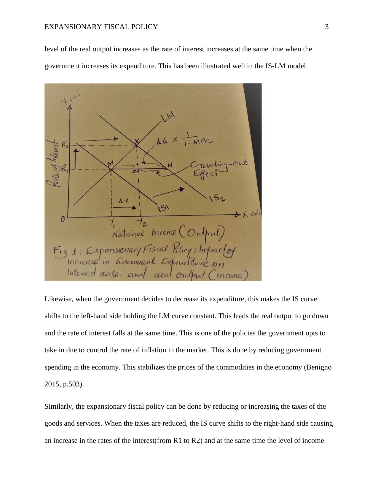
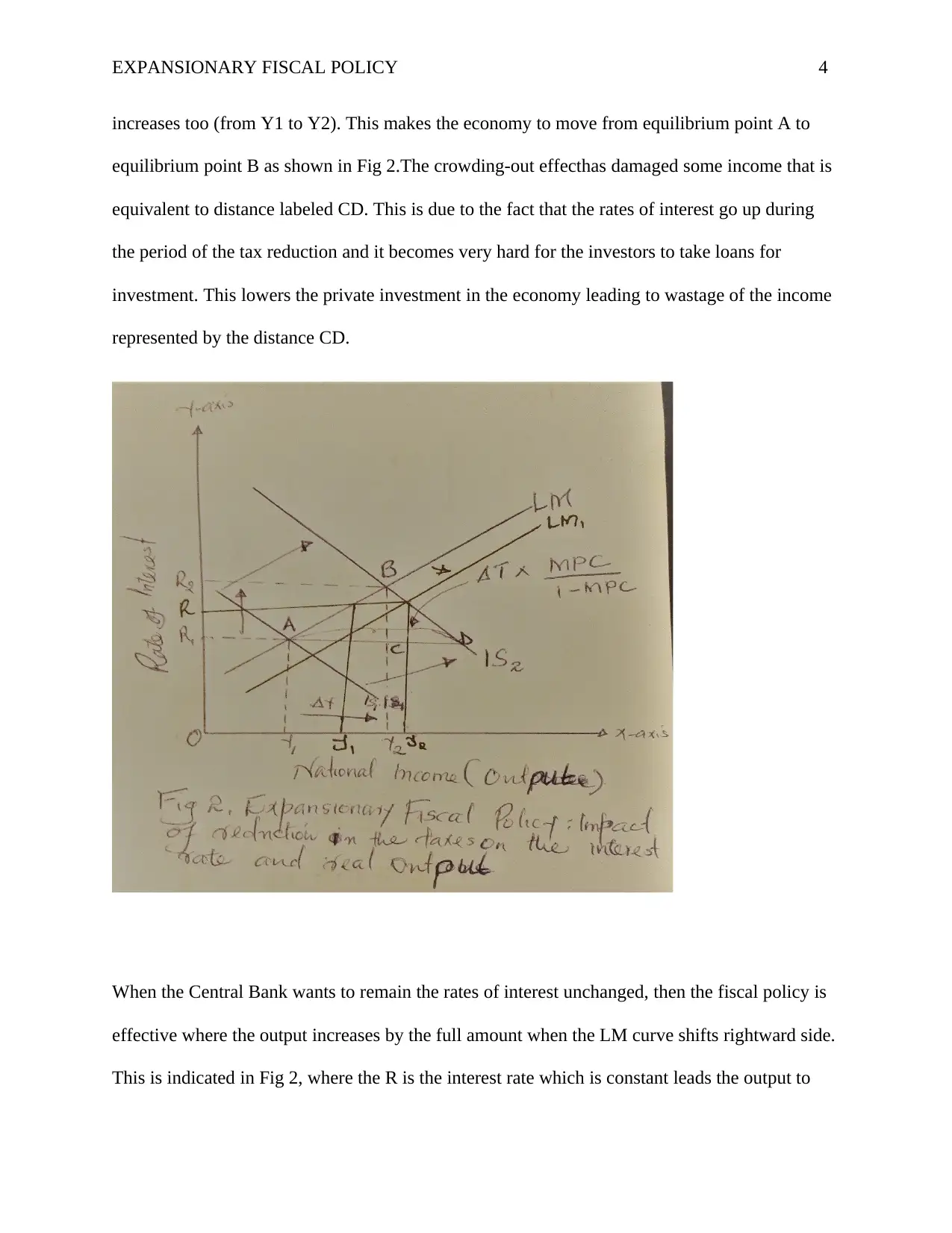
This assignment provides a detailed analysis of expansionary fiscal policy within a closed economy using the IS-LM model. It explains how an increase in government expenditure or a reduction in taxes affects real output and interest rates. The analysis includes diagrams illustrating the shifts in the IS and LM curves and discusses the crowding-out effect. Furthermore, it examines the Central Bank's potential reactions to maintain a constant interest rate. The assignment also addresses the relationship between money demand, output levels, and interest rates, and discusses the impact of nominal wage flexibility on the economy. The document concludes by referencing relevant academic sources, offering a comprehensive overview of the topic. The student document is available on Desklib, a platform offering a variety of study resources.

EXPANSIONARY FISCAL POLICY 1
EXPANSIONARY FISCAL POLICY
Student Name
Institutional Affiliation
Facilitator
Course
Date

EXPANSIONARY FISCAL POLICY 2
Question1
Expansionary fiscal policy is where the government is involved and it requests to increase the
aggregate demand through increasing its expenditure on the level of national income (Eggertsson
2011, p.59). This can be either increasing their spending and/ or reducing the taxes. The
aggregate for the demand for the commodities go up and the IS curve to shift to the right
handwhen the expenditure for the government increases(Afonsoand Sousa 2012, p.4439). In Fig.
1. shows that, when the government increases its expenditure then the IS curve shifts from IS1 to
IS2.
Since the LS curve intersects the IS curves 1 and 2, then the horizontal distance between IS1 and
IS2 curves is equivalent to the government expenditure increaseby its multiplier. That is, change
in government expenditure multiplied by 1/1-MPC which shows the national income increase is
equal to the MN distance as per the model of Keynes’ multiplier. In the IS-LM model, the
Keynesian Multiplier works to cause the MN distance which is not equivalent to the actual
increase in the real outcome (Davigand Leeper2011, p.211). The reason behind this is due to the
fact that the IS curve shifts to the right as the rates of interest rises which leads toa reduction in
the investment of private sectors. TheIS2 curve cuts the LM curve at point X since the LM curve
is held constant at this time. Inthe IS-LM model, when the government increases its expenditure,
then the equilibrium relocates from point M to point X. The rates of interest increase from R1 to
R2 as well as the real output increasing from Y1 to Y2(Nachane2018, p.1).
The distance represented by ZN is the income that has been fallen over because when the rates of
interest go up, the private investment falls down. This income in that distance ZN is what we call
the crowding- out effect that arises after the government increases its expenditure. Therefore, the

EXPANSIONARY FISCAL POLICY 3
level of the real output increases as the rate of interest increases at the same time when the
government increases its expenditure. This has been illustrated well in the IS-LM model.
Likewise, when the government decides to decrease its expenditure, this makes the IS curve
shifts to the left-hand side holding the LM curve constant. This leads the real output to go down
and the rate of interest falls at the same time. This is one of the policies the government opts to
take in due to control the rate of inflation in the market. This is done by reducing government
spending in the economy. This stabilizes the prices of the commodities in the economy (Benigno
2015, p.503).
Similarly, the expansionary fiscal policy can be done by reducing or increasing the taxes of the
goods and services. When the taxes are reduced, the IS curve shifts to the right-hand side causing
an increase in the rates of the interest(from R1 to R2) and at the same time the level of income

EXPANSIONARY FISCAL POLICY 4
increases too (from Y1 to Y2). This makes the economy to move from equilibrium point A to
equilibrium point B as shown in Fig 2.The crowding-out effecthas damaged some income that is
equivalent to distance labeled CD. This is due to the fact that the rates of interest go up during
the period of the tax reduction and it becomes very hard for the investors to take loans for
investment. This lowers the private investment in the economy leading to wastage of the income
represented by the distance CD.
When the Central Bank wants to remain the rates of interest unchanged, then the fiscal policy is
effective where the output increases by the full amount when the LM curve shifts rightward side.
This is indicated in Fig 2, where the R is the interest rate which is constant leads the output to

EXPANSIONARY FISCAL POLICY 5
increase from y1 to y2. This increase is justified by the increase in the supply of money in the
short-run (Auerbachand Gorodnichenko2012, p.1).
Question2
Disagree. The reason behind this is due to the fact that the output level goes up when the money
demand is higher than in the changes in the rates of interest. This is due to the fact of the effect
of the expansionary fiscal policy in the economy (Precious and Kosi2014, p.76). when the
demand for money is high it leads the LM curve to shift to the right as shown in Fig 3.
In this case, the output is high as the money demand goes up at the same time. This is because
ofincome increases as the demand for the precautionary increase. When the rates of the interest
go down, the demand for the speculative increases too (Fioreand Tristani 2012, p.906). Thus,
interest rate declines from r1 to r2, then the precautionary demand and speculative demand

EXPANSIONARY FISCAL POLICY 6
increases. Thus,the total demand for money increases.The equilibrium moves from point E to a
new equilibrium E2 as the LM curve moves to curve LM1. This is because of the increase in
money demand which leads the interest rate to increase.
At this equilibrium point E2, the equilibrium income is high while the interest rate also goes
down. This indicates that the output level rises with the money demand going up and the interest
rates go down at the same time. So, the statement should be correct if the output is very large
with rising in the demand formoney (Summers 2014, p.65).
Question3
i. Nominal wages are fully flexible.
The economy is atthe potential output when the aggregate demand and the aggregate supply
models are predicted in the country.Reducing the governmentexpenditure, the aggregate
equilibrium curve goes down thus decreasing the real output. Therefore, the investment or saving
curve will shift backwarddue to a low real output which leads to fewer savings caused by the rate
of interest going up. This causes the price level to go up as the real wage rate decrease when the
nominal wages attained stability. In long run, no effect on the real output which can be caused by
the level of prices because price level change will not affect the amount of the factors of
production in the economy (Jacobs and Rush 2015, p.9).
The level of the output produced in the economy by the firms, in the long run, is related to the
level of prices in the long-run aggregate supply curve. Employment reaches its natural level
under only one single real wage. This single real wage generates natural employment. This is
achieved through a combination of the infinity huge set of nominal wage and level of prices. At

EXPANSIONARY FISCAL POLICY 7
this level, the prices increase as it requires additional nominal wages that lead tothe creation of a
real wage rate where the nominal wages will be flexible.
One output level is given out in the economy at any level of the prices. The real output remains
constant as the price level go up as well asthe level of price go down during the long run
equilibrium.
ii. Nominal wages are relatively slow to adjust.
Most of the long-term contracts work in the firms when the nominal wage in slowly adjustable in
the economy. Most of the prices in the economy go up due to a decrease in the supply of the
commodities in the market in the short run. The real output in the short run is greater than the
level of prices in the economy as a fact of the aggregate demand. This is due to constant in the
real wages since the factors inputs prices do not increase much. However, when output continues
to increase, the economy expands as it moves relative to the full capacity. The quantity of the
output in the economy will go down as the prices start climbing up rapidly (Blanchard,
Jaumotteand Loungani2014, p.2).
iii. Nominal wages are completely rigid.
The stickiness of wage indicates that the economy may be having some challenges when
operating at potential (Woodford 2011, p.1). Fairly,in the short run, the economy is in a position
to operate either above or below potential output. this corresponds that, the overall
unemployment rate can be below or above the natural level.
The equilibrium is checked through the market where its conditions are observed keenly in the
level of the prices so as the equilibrium is not lost at all but regained. Nominal wages in the
economy can be sticky because of their relationship with the rate of unemployed people, interest

EXPANSIONARY FISCAL POLICY 8
rate and other prices of commodities that might be sticky. Wage gets a fix nominal wages for the
life of the contract since there is variation in the length of the contracts in the temporary
employees.
Having the existence of contracts in the economy, the firms and the employees accept some of
the wages at the time of negotiation assuming that the conditions for the economy may change as
the agreement is in place. The employers and employees should be ready to learn the conditions
in the market so as they can put good measures on how to deal with the cost of living in the
economy. Most of the cases, unions are involved with the negotiations whereby they waste a lot
of time without doing something that can be productive in the market. These negations are
costly.The most important thing for the workers is to know that their nominal wages will be
fixed for some period of time.
Majority of the part-time employees find it hard to challenge most of the economic conditions
such as inflation and adjusting with the cost of living. One might think they have a better life but
not the case due to their nominal wages. Most of the firms are not concerned with the aggregate
prices level where it rises so high creating inflation in the country hence leading to a hard life for
the part-time employees. The cost of living becomes so challenging at the same time when prices
are high.

EXPANSIONARY FISCAL POLICY 9
Reference
Afonso, A. and Sousa, R.M., 2012. The macroeconomic effects of fiscal policy. Applied
Economics, 44(34), pp.4439-4454.
Auerbach, A.J. and Gorodnichenko, Y., 2012. Measuring the output responses to fiscal policy.
American Economic Journal: Economic Policy, 4(2), pp.1-27.
Benigno, P., 2015. New-Keynesian Economics: An AS-AD View. Research in Economics,
69(4), pp.503-524.
Blanchard, O.J., Jaumotte, F. and Loungani, P., 2014. Labor market policies and IMF advice in
advanced economies during the Great Recession. IZA Journal of Labor Policy, 3(1), p.2.
David, T. and Leeper, E.M., 2011. Monetary-fiscal policy interactions and fiscal stimulus.
European Economic Review, 55(2), pp.211-227.
Eggertsson, G.B., 2011. What fiscal policy is effective at zero interest rates?NBER
Macroeconomics Annual, 25(1), pp.59-112.
Fiore, F.D. and Tristani, O., 2012. Optimal monetary policy in a model of the credit channel. The
Economic Journal, 123(571), pp.906-931.
Jacobs, D. and Rush, A., 2015. Why is wage growth so low?RBA Bulletin, June, pp.9-18.
Nachane, D.M., 2018. Keynesian Economics: Brief Overview. In Critique of the New Consensus
Macroeconomics and Implications for India (pp. 1-38). Springer, New Delhi.
Precious, C. and Makhetha-Kosi, P., 2014. Impact of monetary policy on economic growth: a
case study of South Africa. Mediterranean journal of social sciences, 5(15), p.76.
Summers, L.H., 2014. US economic prospects: Secular stagnation, hysteresis, and the zero-lower
bound. Business Economics, 49(2), pp.65-73.

EXPANSIONARY FISCAL POLICY 10
Woodford, M., 2011. The simple analytics of government expenditure multiplier. American
Economic Journal: Macroeconomics, 3(1), pp.1-35.