BUS1BAN Statistics Project: Analysis of Student Mobile Phone Usage

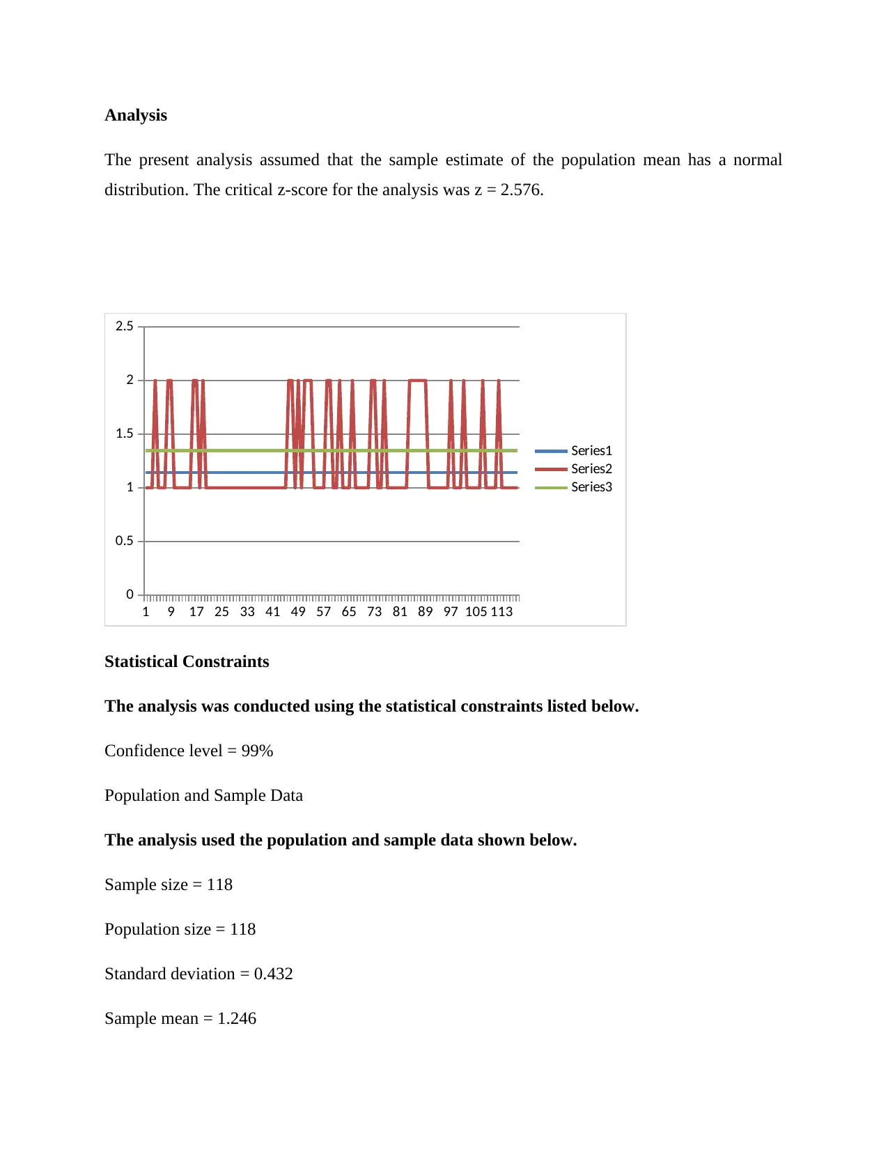
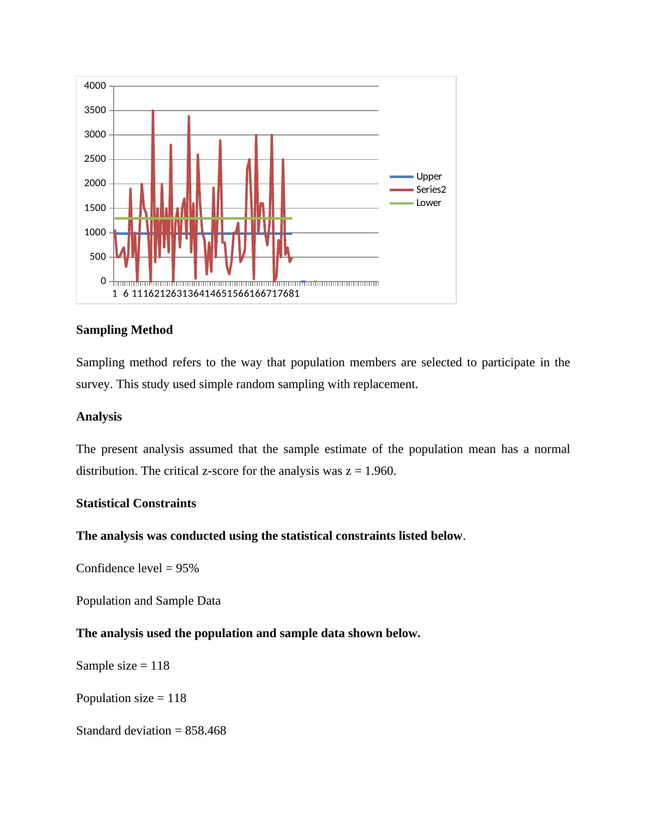
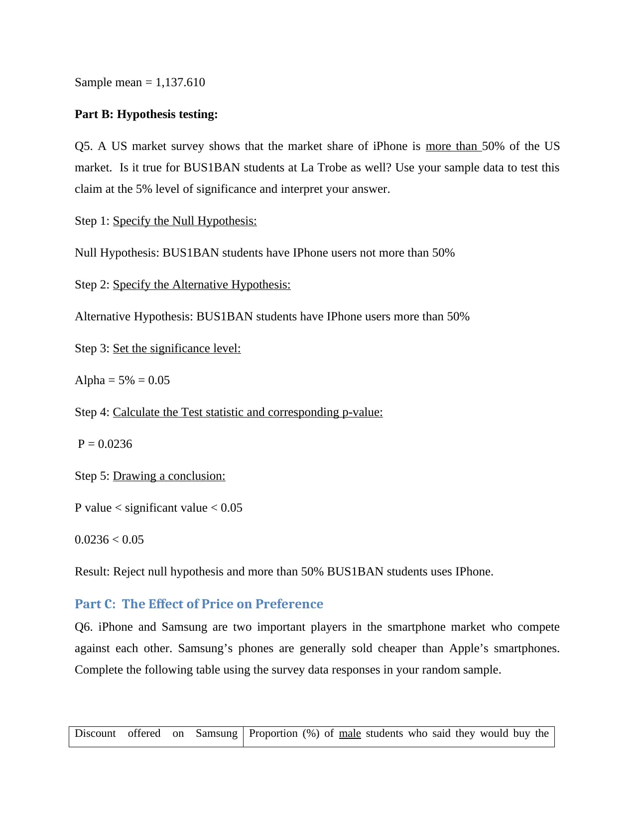
This statistics project analyzes student mobile phone usage within the BUS1BAN class at La Trobe University. The project begins with a description of the sampling plan employed, followed by an analysis of descriptive statistics, including gender proportions, cross-classification tables of mobile phone brands and gender, and the relationship between earnings and mobile phone spending. The analysis continues with inferential statistics, including point estimates, confidence intervals for iPhone users and average monthly earnings, and hypothesis testing regarding iPhone market share among students. The project also explores the effect of price on preference, using linear regression to analyze the relationship between discounts on Samsung phones and the proportion of male students who would purchase them. The project concludes with key findings and interpretations of the statistical results, including the relationships between variables and the implications of the analysis.

Research Project

SECTION 1
PART A: Sampling
Q1. What sampling plan did you employ to select your sample?
Random sampling has been employed to select sample of the given hypothesis.
Q2. Apart from the sampling plan you employed to select your random sample, use your own
words to briefly describe two other commonly used sampling plans that were discussed in the
workshops?
Stratified Sampling
Stratified Sampling requires a great deal of thought and organization, but the use of increasingly
complex procedures yields increasingly precise results. If it is possible to identify subgroups
within a larger population, the thinking behind the study described is to monitor these collections
free of each other.
Systematic sampling
Systematic sampling uses a structure for the validation procedure, but it is an optional structure
of your decision. By implementing an expected option plan, you can update your example. In
any event, given that the plans implemented are in the personal testing process, it is also possible
to end up with a non-delegated test. Despite everything, you may not get information about the
agent.
Part B: Descriptive Statistics
Q3. Analysis on gender proportion:
a. In the following table, report proportion of the students based on gender in your sample.
Gender Sample Proportion (in percentage form)
Female 62

Male 56
b. Use an appropriate chart (properly labeled) to display information in Q3-a above and provide
brief interpretation on the chart.
53%
47%
Total
Female Male
Interpretation: In the above sample total 47% participants are female and 53% are males.
Q4. Investigating the relationship between mobile phone brands and student gender:
a. Complete the following cross classification table of frequencies.
Brand
Apple Samsung LG
Basic
mobile
phone
Other
smart
phone
Do not
use
mobile
phone Total
Gender
Male 38 13 1 0 4 0 56
Female 51 9 0 0 2 0 62
Total 89 22 1 0 6 0 118

b. Derive row relative frequencies in the following table based on cross classification table of
frequencies in Q4-a above.
Brand
Apple Samsung LG
Basic
mobile
phone
Other
smart
phone
Do not
use
mobile
phone Total
Gender
Male 0.67 0.23 0.017 0 0.071 0 1
Female 0.84 0.14 0 0 0.032 0 1
Total 1.51 0.37 0.017 0 0.103 0 1
c. Use an appropriate graph to display row relative frequencies contained in the above cross-
classification table. Briefly discuss whether there is a relationship between gender and mobile
phone brands.
Apple Samsung LG Basic
mobile
phone
Other
smart
phone
Do not use
mobile
phone
0.00
0.10
0.20
0.30
0.40
0.50
0.60
0.70
0.80
0.90
Male
Female

The above bar chart shows that females are more attracted towards brand than boys. Boys are
ready to use other smartphones but females are not; as the graph indicates that Apple brand is has
high proportion of female than males and other brands like Samsung and LG is lead by boys.
Q5. Investigating the relationship between earnings and money spent on mobile phone by
gender:
a. In the following table, report average monthly earnings and mobile bill of students by gender
in your sample.
Female Male
Average Monthly Earnings ($) 1117.06 1160.35
Average Monthly Bill ($) 63.17 65.14
b. Produce a scatter plot (showing trend line, linear equation and R square) using Excel, to show
the relationship between earnings and money spent on mobile phone for each gender.
0 200 400 600 800 1000 1200
0
200
400
600
800
1000
1200
1400
65.14
Chart Title
Series2
Linear (Series2)
Axis Title
Axis Title
Q6. Descriptive statistics on the relationship between average monthly earning and average
monthly mobile bill by gender:

a. Use Excel and fill in the table. Provide the following statistical measures to examine the
relationship between average monthly earning and average monthly mobile bill.
Female Male
Covariance 21.5 21.5
Coefficient of Correlation 0.2212 0.09
Coefficient of Determination 0.0489 0.081
Y-intercept 0.01077X + 51.1409 0.00373X + 60.81322
Slope 0.01077 0.00373
Least Squares Line 0.01077X + 51.1409 0.00373X + 60.81322
b)
Female:
 Covariance: The result shows that females are not associated with income and bill paid.
 Coefficient of Correlation: The result shows value of coefficient of correlation much less
than one; this indicates that there is no association between income and bill paid.
 Coefficient of Determination: It is the square of correlation and hence showing the
same conclusion.
 Y-Intercept: the intercept of both bill paid and income of female is at point 0.01077
 Slope: The variable is showing positive slope between bills paid and income received.
Male:
 Covariance: The result shows that females are not associated with income and bill paid.
 Coefficient of Correlation: The result shows value of coefficient of correlation much less
than one; this indicates that there is no association between income and bill paid.
 Coefficient of Determination: It is the square of correlation and hence showing the
same conclusion.

 Y-Intercept: the intercept of both bill paid and income of female is at point 0.00373
 Slope: The variable is showing positive slope between bills paid and income received
Part C: Summary and Discussion
Q7. Briefly discuss how to determine the relationship between two nominal variables, and
how to determine the relationship between two numerical variables.
a. Relationship between two nominal variables
The nominal variable relationship refers to the relationship or relationships that can be measured
on observable factors. Intangible factors are factors considered high and which do not have a
natural environment. Measurements of overlapping factors that are generally evaluated in
sociological tests include sexual orientation, race, close affiliation and elementary school. Cross
organization (also known as a skill table or variable) is generally used to test the link between
tangible factors. The Chi Square independence test is generally used to determine the links
between two factors to evaluate the supernatural self.
b. Relationship between two numerical variables:
Statistical reports are the ones we will focus on in this class. In this type of relationship, mixing
from the example is normal. If we know the estimate of one variable, we can make a consistent
estimate of the other variable. In any event, this is just an estimate.
When a straight line summarizes the relationship between two numerical factors, we affirm that
the two factors are either directly related or that the two factors are directly related.
Q8. What are your main findings based on the analysis in Q3-Q6 of Part B?
There is positive relationship between Male and female and their average bill and average
income.

SECTION-2: INFERENTIAL STATISTICS
Part A: Point Estimate and Confidence Interval
Q1. Suppose you randomly select a student from BUS1BAN class, how likely is it that the
student selected will be a female student? How likely is it that the student selected will be an
IPhone user?
Proportion in percentage form ( ^p)
Female students 25%
iPhone users 80%
Q2. Estimate the 99% confidence interval for the proportion of iPhone users. Show the
confidence intervals graphically and interpret your results. You should show the formula and
calculation by putting values in the formula.
Margin of error = 0.103
Other findings that emerged from the analysis appear below:
Sample estimate of population total = 147.000
Confidence interval = 1.143 to 1.348
Standard error = 0.040
Methodology
This section describes the assumptions, sampling method, analytical procedures, and data inputs
that were used by the Sample Size Calculator to produce the findings shown above.
Sampling Method
Sampling method refers to the way that population members are selected to participate in the
survey. This study used simple random sampling with replacement.

Analysis
The present analysis assumed that the sample estimate of the population mean has a normal
distribution. The critical z-score for the analysis was z = 2.576.
1 9 17 25 33 41 49 57 65 73 81 89 97 105 113
0
0.5
1
1.5
2
2.5
Series1
Series2
Series3
Statistical Constraints
The analysis was conducted using the statistical constraints listed below.
Confidence level = 99%
Population and Sample Data
The analysis used the population and sample data shown below.
Sample size = 118
Population size = 118
Standard deviation = 0.432
Sample mean = 1.246

Q3. What are the average monthly earnings of male and female students in your sample?
Average monthly earnings in dollars ($)
Female students 1117.06 1160.35
Male students 1160
Q4. Provide 95% confidence interval of the average monthly earnings for each gender. Show the
confidence intervals graphically and interpret your answer. You should show the formula and
calculation by putting values in the formula.
The main goal of the present analysis is to find the margin of error, given a sample size of 118
and a confidence level of 95%.
Here is the answer to that question:
Margin of error = 154.893
Other findings that emerged from the analysis appear below:
Sample estimate of population total = 134,238.000
Confidence interval = 982.717 to 1,292.503
Standard error = 79.028
Methodology
This section describes the assumptions, sampling method, analytical procedures, and data inputs
that were used by the Sample Size Calculator to produce the findings shown above.

1 6 111621263136414651566166717681
0
500
1000
1500
2000
2500
3000
3500
4000
Upper
Series2
Lower
Sampling Method
Sampling method refers to the way that population members are selected to participate in the
survey. This study used simple random sampling with replacement.
Analysis
The present analysis assumed that the sample estimate of the population mean has a normal
distribution. The critical z-score for the analysis was z = 1.960.
Statistical Constraints
The analysis was conducted using the statistical constraints listed below.
Confidence level = 95%
Population and Sample Data
The analysis used the population and sample data shown below.
Sample size = 118
Population size = 118
Standard deviation = 858.468

Sample mean = 1,137.610
Part B: Hypothesis testing:
Q5. A US market survey shows that the market share of iPhone is more than 50% of the US
market. Is it true for BUS1BAN students at La Trobe as well? Use your sample data to test this
claim at the 5% level of significance and interpret your answer.
Step 1: Specify the Null Hypothesis:
Null Hypothesis: BUS1BAN students have IPhone users not more than 50%
Step 2: Specify the Alternative Hypothesis:
Alternative Hypothesis: BUS1BAN students have IPhone users more than 50%
Step 3: Set the significance level:
Alpha = 5% = 0.05
Step 4: Calculate the Test statistic and corresponding p-value:
P = 0.0236
Step 5: Drawing a conclusion:
P value < significant value < 0.05
0.0236 < 0.05
Result: Reject null hypothesis and more than 50% BUS1BAN students uses IPhone.
Part C: The Effect of Price on Preference
Q6. iPhone and Samsung are two important players in the smartphone market who compete
against each other. Samsung’s phones are generally sold cheaper than Apple’s smartphones.
Complete the following table using the survey data responses in your random sample.
Discount offered on Samsung Proportion (%) of male students who said they would buy the