Economics Assignment: Analyzing Labor Demand and Supply Dynamics

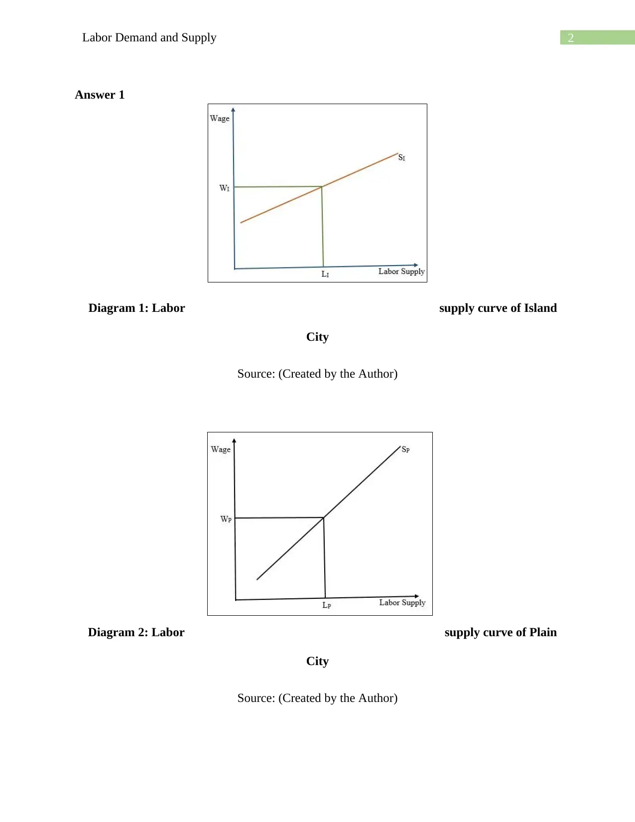
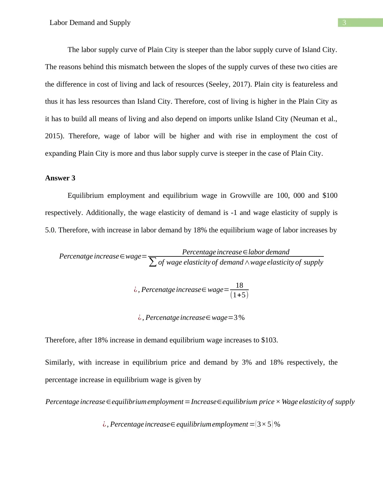
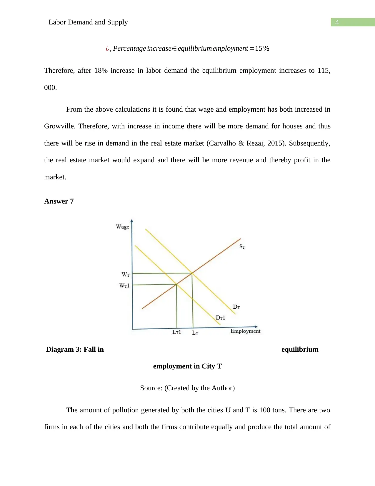
This economics assignment delves into the dynamics of labor demand and supply, examining factors that influence labor market equilibrium. The analysis includes graphical representations of labor supply curves in different city contexts, exploring how cost of living and resource availability impact wage and employment levels. The assignment further explores the effects of changes in labor demand on equilibrium wage and employment, utilizing concepts of wage elasticity. It investigates how changes in income and labor demand affect the real estate market. Additionally, the assignment examines the impact of pollution on labor supply, analyzing how tax policies implemented to reduce pollution affect equilibrium employment levels in two different cities, comparing the outcomes in each city. The solution includes diagrams and references to support the analysis.

Running head: Labor Demand and Supply
Labor Demand and Supply
Name of the Student
Name of the University
Student ID

1Labor Demand and Supply
Table of Contents
Answer 1..........................................................................................................................................2
Answer 3..........................................................................................................................................3
Answer 7..........................................................................................................................................4
Reference.........................................................................................................................................6

2Labor Demand and Supply
Answer 1
Diagram 1: Labor supply curve of Island
City
Source: (Created by the Author)
Diagram 2: Labor supply curve of Plain
City
Source: (Created by the Author)

3Labor Demand and Supply
The labor supply curve of Plain City is steeper than the labor supply curve of Island City.
The reasons behind this mismatch between the slopes of the supply curves of these two cities are
the difference in cost of living and lack of resources (Seeley, 2017). Plain city is featureless and
thus it has less resources than Island City. Therefore, cost of living is higher in the Plain City as
it has to build all means of living and also depend on imports unlike Island City (Neuman et al.,
2015). Therefore, wage of labor will be higher and with rise in employment the cost of
expanding Plain City is more and thus labor supply curve is steeper in the case of Plain City.
Answer 3
Equilibrium employment and equilibrium wage in Growville are 100, 000 and $100
respectively. Additionally, the wage elasticity of demand is -1 and wage elasticity of supply is
5.0. Therefore, with increase in labor demand by 18% the equilibrium wage of labor increases by
Percenatge increase∈wage= Percentage increase∈labor demand
∑ of wage elasticity of demand∧wage elasticity of supply
¿ , Percenatge increase∈ wage= 18
(1+5)
¿ , Percenatge increase∈wage=3 %
Therefore, after 18% increase in demand equilibrium wage increases to $103.
Similarly, with increase in equilibrium price and demand by 3% and 18% respectively, the
percentage increase in equilibrium wage is given by
Percentage increase ∈equilibrium employment =Increase∈equilibrium price × Wage elasticity of supply
¿ , Percentage increase∈ equilibrium employment = ( 3× 5 ) %

4Labor Demand and Supply
¿ , Percentage increase∈equilibrium employment =15 %
Therefore, after 18% increase in labor demand the equilibrium employment increases to 115,
000.
From the above calculations it is found that wage and employment has both increased in
Growville. Therefore, with increase in income there will be more demand for houses and thus
there will be rise in demand in the real estate market (Carvalho & Rezai, 2015). Subsequently,
the real estate market would expand and there will be more revenue and thereby profit in the
market.
Answer 7
Diagram 3: Fall in equilibrium
employment in City T
Source: (Created by the Author)
The amount of pollution generated by both the cities U and T is 100 tons. There are two
firms in each of the cities and both the firms contribute equally and produce the total amount of

5Labor Demand and Supply
pollution. It means the firms in cities U and T generate 50 tons of pollution each. City T
implements a tax policy to reduce the pollution and owing to that the firms in the city has to
reduce their production. Consequently, the pollution of City T reduced by 20% to 80 tons (Hanna
& Oliva, 2015). However, the equilibrium employment reduced by (LT-LT1) as shown in diagram
3. Similarly, City U also implemented the same policy to reduce pollution. It is observed that in
City U that each of the two firms reduced pollution by 20% that means each now produces 40
tons of pollution. It implies that City U produces 80 tons of pollution in total which is similar as
City T. Thus, it can be inferred that equilibrium employment in City U has reduced by the
amount equal to (LT-LT1).

6Labor Demand and Supply
Reference
Carvalho, L., & Rezai, A. (2015). Personal income inequality and aggregate demand. Cambridge
Journal of Economics, 40(2), 491-505.
Hanna, R., & Oliva, P. (2015). The effect of pollution on labor supply: Evidence from a natural
experiment in Mexico City. Journal of Public Economics, 122, 68-79.
Neuman, T., Cubanski, J., Huang, J., & Damico, A. (2015). The rising cost of living
longer. Kaiser Family Foundation. www. kff. org/medicare/report/the-rising-cost-of-
living-longer-analysis-ofmedicare-spending-by-age-for-beneficiaries-in-traditional-
medicare.
Seeley, K. (2017). Short-Run Aggregate Supply/Aggregate Demand and Policy.
In Macroeconomics in Ecological Context (pp. 273-294). Springer, Cham.