Master's Economics: Labour Supply, Firm Production, Goods Analysis
VerifiedAdded on 2023/01/18
|14
|2654
|67
Homework Assignment
AI Summary
This economics assignment delves into core economic principles through a series of questions and answers. The assignment begins with an analysis of Ann's labour supply, constructing her budget constraint and indifference curves to determine her optimal consumption-leisure mix, including the impact of wage increases using income-substitution effects. The f(K, L) model is then employed to explore how firms should choose capital and labour inputs, detailing assumptions about the production function. Finally, the assignment examines consumption patterns of tea and coffee to classify them as normal or inferior goods, utilizing income and substitution effects to explain the consumption behavior. The document provides a detailed analysis of each question, supported by graphs and economic concepts.

QUESTIONS AND
ANSWERS ON LABOUR
SUPPLY, FIRM
PRODUCTIONS AND
NORMAL AND INFERIOR
GOOD
ANSWERS ON LABOUR
SUPPLY, FIRM
PRODUCTIONS AND
NORMAL AND INFERIOR
GOOD
Paraphrase This Document
Need a fresh take? Get an instant paraphrase of this document with our AI Paraphraser
Table of Contents
INTRODUCTION...........................................................................................................................3
MAIN BODY..................................................................................................................................3
Question 1........................................................................................................................................3
Equation of Budget Constraint and its representation.................................................................3
Consumption-Leisure Diagram and MRS...................................................................................4
Income-Substitution effects.........................................................................................................5
Question 2........................................................................................................................................6
Use of f (K, L) model..................................................................................................................6
Question 3......................................................................................................................................10
Consumption of Tea..................................................................................................................10
Consumption of Coffee..............................................................................................................11
CONCLUSION..............................................................................................................................12
REFERENCES................................................................................................................................1
INTRODUCTION
Economics and various concepts associated with it are extremely important in analysing
the current and future trends thus giving a better view point. In the present report, concepts such
as Budget Constraints, Indifference curve, Production function, and Income Substitution effect
will be analysed with respect to different questions that have been raised in the case study and
the answers will be supported by appropriate charts, figures and concepts thus giving reasonable
answers and conclusions.
MAIN BODY
Question 1
Equation of Budget Constraint and its representation
The concept of budget constraint helps in determining that what is the maximum budget
line or amount of an individual consumer that he is willing to spend in order to consume a
combination of goods or services within the given amount (Miller, Bergtold and Featherstone,
2019). A preference map along with budget constraint is used to analyse that what will be the
preference of the consumer amongst various goods and services that are available as options for
the consumer.
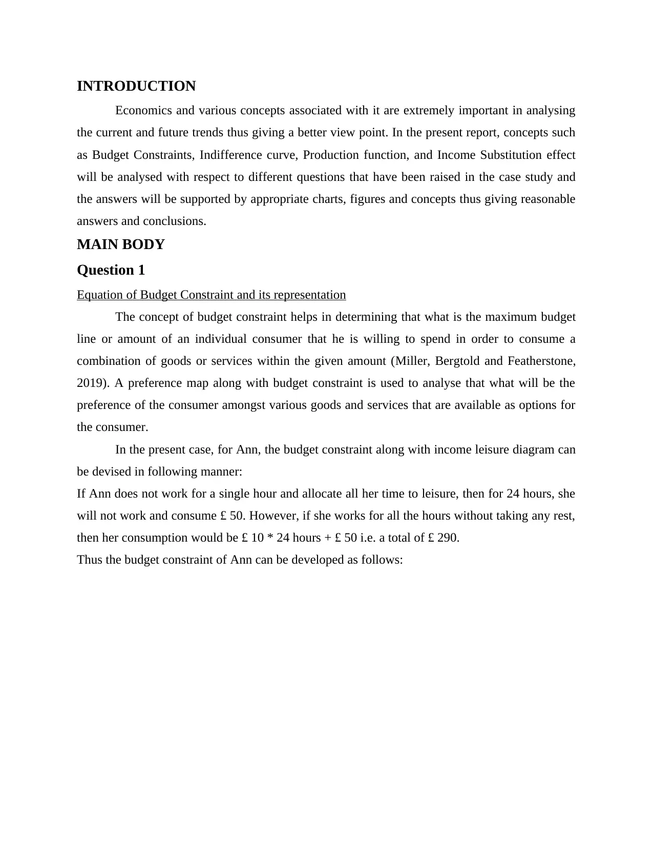
In the present case, for Ann, the budget constraint along with income leisure diagram can
be devised in following manner:
If Ann does not work for a single hour and allocate all her time to leisure, then for 24 hours, she
will not work and consume £ 50. However, if she works for all the hours without taking any rest,
then her consumption would be £ 10 * 24 hours + £ 50 i.e. a total of £ 290.
Thus the budget constraint of Ann can be developed as follows:
Economics and various concepts associated with it are extremely important in analysing
the current and future trends thus giving a better view point. In the present report, concepts such
as Budget Constraints, Indifference curve, Production function, and Income Substitution effect
will be analysed with respect to different questions that have been raised in the case study and
the answers will be supported by appropriate charts, figures and concepts thus giving reasonable
answers and conclusions.
MAIN BODY
Question 1
Equation of Budget Constraint and its representation
The concept of budget constraint helps in determining that what is the maximum budget
line or amount of an individual consumer that he is willing to spend in order to consume a
combination of goods or services within the given amount (Miller, Bergtold and Featherstone,
2019). A preference map along with budget constraint is used to analyse that what will be the
preference of the consumer amongst various goods and services that are available as options for
the consumer.
In the present case, for Ann, the budget constraint along with income leisure diagram can
be devised in following manner:
If Ann does not work for a single hour and allocate all her time to leisure, then for 24 hours, she
will not work and consume £ 50. However, if she works for all the hours without taking any rest,
then her consumption would be £ 10 * 24 hours + £ 50 i.e. a total of £ 290.
Thus the budget constraint of Ann can be developed as follows:
⊘ This is a preview!⊘
Do you want full access?
Subscribe today to unlock all pages.
Trusted by 1+ million students worldwide
It can therefore be concluded that if Ann works for entire 24 hours in a day incessantly, then she
will be able to spend as much as £ 290 and if she does not work for a single hour and rest for the
entire day, then the maximum amount that she can spend is £ 50 which is her non labour income.
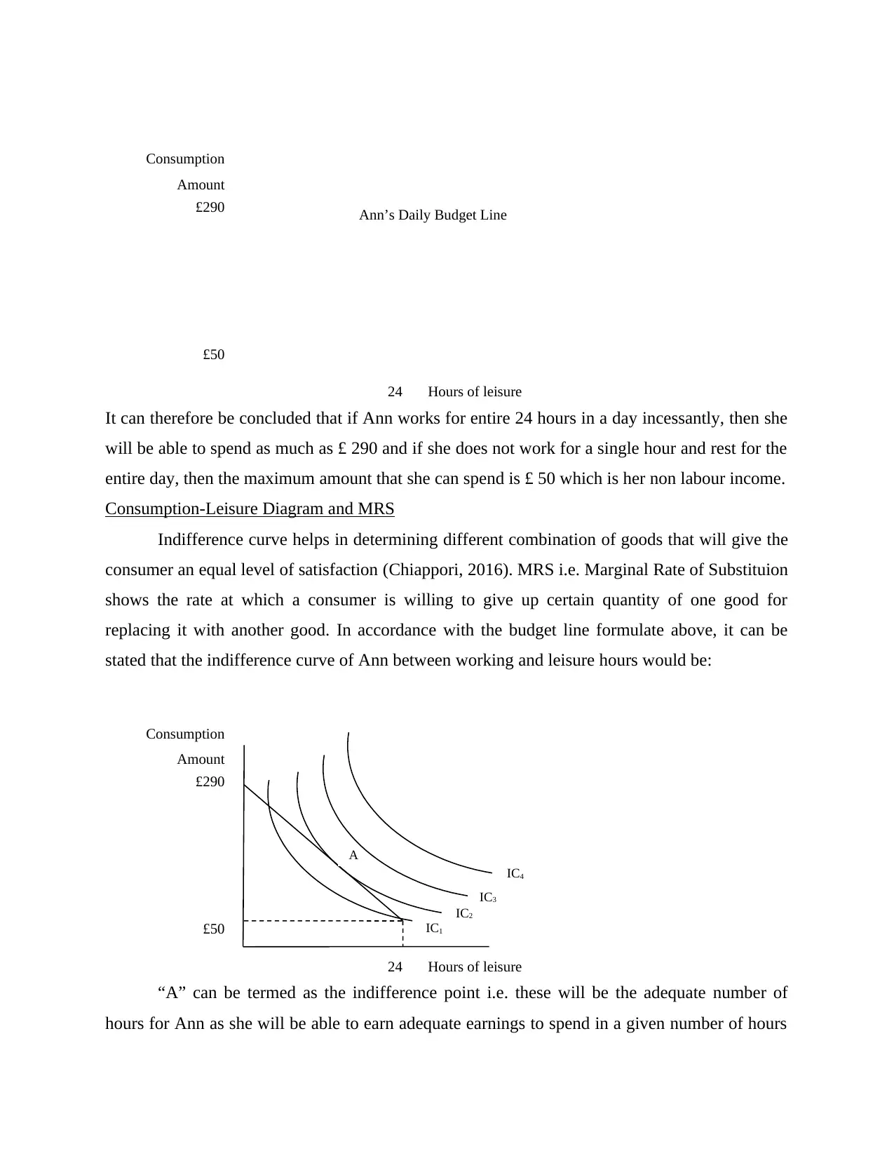
Consumption-Leisure Diagram and MRS
Indifference curve helps in determining different combination of goods that will give the
consumer an equal level of satisfaction (Chiappori, 2016). MRS i.e. Marginal Rate of Substituion
shows the rate at which a consumer is willing to give up certain quantity of one good for
replacing it with another good. In accordance with the budget line formulate above, it can be
stated that the indifference curve of Ann between working and leisure hours would be:
“A” can be termed as the indifference point i.e. these will be the adequate number of
hours for Ann as she will be able to earn adequate earnings to spend in a given number of hours
24 Hours of leisure
£50
£290
Consumption
Amount
Ann’s Daily Budget Line
24 Hours of leisure
£50
£290
Consumption
Amount
IC1
A
IC2
IC3
IC4
will be able to spend as much as £ 290 and if she does not work for a single hour and rest for the
entire day, then the maximum amount that she can spend is £ 50 which is her non labour income.
Consumption-Leisure Diagram and MRS
Indifference curve helps in determining different combination of goods that will give the
consumer an equal level of satisfaction (Chiappori, 2016). MRS i.e. Marginal Rate of Substituion
shows the rate at which a consumer is willing to give up certain quantity of one good for
replacing it with another good. In accordance with the budget line formulate above, it can be
stated that the indifference curve of Ann between working and leisure hours would be:
“A” can be termed as the indifference point i.e. these will be the adequate number of
hours for Ann as she will be able to earn adequate earnings to spend in a given number of hours
24 Hours of leisure
£50
£290
Consumption
Amount
Ann’s Daily Budget Line
24 Hours of leisure
£50
£290
Consumption
Amount
IC1
A
IC2
IC3
IC4
Paraphrase This Document
Need a fresh take? Get an instant paraphrase of this document with our AI Paraphraser
amongst all the Indifference Curve’s that could be drawn. Therefore the optimal choice for her
will be to work for 18 hours where she will be able to earn £ 180 + £ 50 i.e. £ 230.
In order to determine her optimal consumption and leisure mix, the MRS can be equated to the
wage:
C = 50 + 10 (24-L) and w = MRS and MRS = C – 180/ L – 18
Therefore,
10 = {50 + 10 (24-L)} – 180/ (L - 18)
10L – 180 = 50 + 240 – 10L
20L = 110
L= 5.5 i.e. Ann would prefer to leisure for 5.5 hours and work for 18.5 hours i.e. earn £50 +
£10(18.5) = £235 which will be optimal earnings for her.
Income-Substitution effects
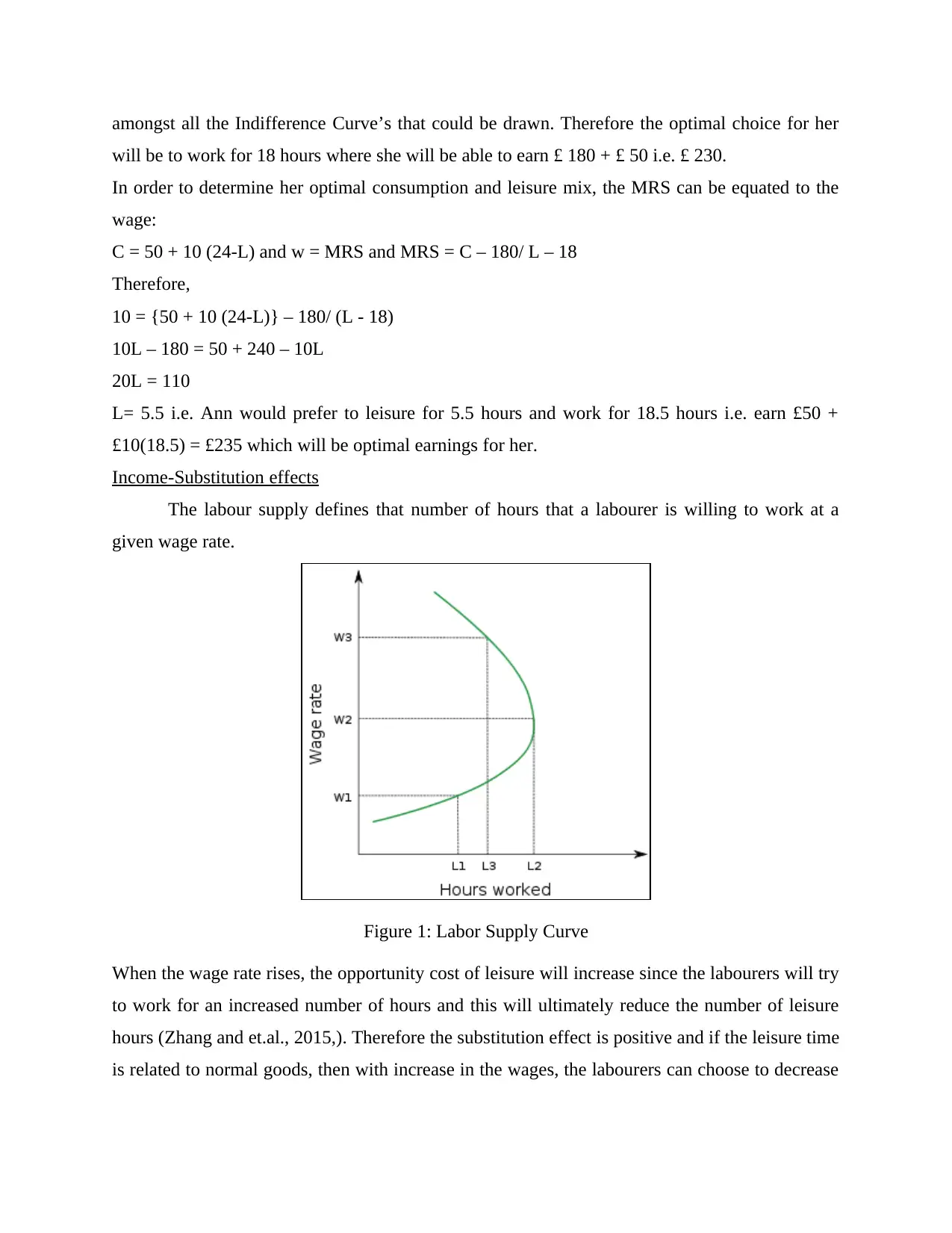
The labour supply defines that number of hours that a labourer is willing to work at a
given wage rate.
Figure 1: Labor Supply Curve
When the wage rate rises, the opportunity cost of leisure will increase since the labourers will try
to work for an increased number of hours and this will ultimately reduce the number of leisure
hours (Zhang and et.al., 2015,). Therefore the substitution effect is positive and if the leisure time
is related to normal goods, then with increase in the wages, the labourers can choose to decrease
will be to work for 18 hours where she will be able to earn £ 180 + £ 50 i.e. £ 230.
In order to determine her optimal consumption and leisure mix, the MRS can be equated to the
wage:
C = 50 + 10 (24-L) and w = MRS and MRS = C – 180/ L – 18
Therefore,
10 = {50 + 10 (24-L)} – 180/ (L - 18)
10L – 180 = 50 + 240 – 10L
20L = 110
L= 5.5 i.e. Ann would prefer to leisure for 5.5 hours and work for 18.5 hours i.e. earn £50 +
£10(18.5) = £235 which will be optimal earnings for her.
Income-Substitution effects
The labour supply defines that number of hours that a labourer is willing to work at a
given wage rate.
Figure 1: Labor Supply Curve
When the wage rate rises, the opportunity cost of leisure will increase since the labourers will try
to work for an increased number of hours and this will ultimately reduce the number of leisure
hours (Zhang and et.al., 2015,). Therefore the substitution effect is positive and if the leisure time
is related to normal goods, then with increase in the wages, the labourers can choose to decrease
the number of working hours thus minimising the number of hours worked and increase the
leisure time.
Question 2
Use of f (K, L) model
The f (K, L) model i.e. the production function is a relationship between the fixed and
variable unis of inputs with that of the output. This concept of economics that helps in
determining the effective efficiency levels of the productivity of a particular unit, help in
ascertain the relationship between Average product, Marginal product and Total product. The
production function and the graph formulated henceforth, assists the managers and production
heads of the company in ascertaining the correct level of the various labour units and capital
units that are to be used in order to attain maximum level of productions i.e. the optimum use of
resources in order to generate maximum production.
The inputs that are used in production function are also termed as factors of production
and these primary factors basically include land, labour and capital but later on entrepreneurship
was also added on as a factor of production i.e. an input. Land which is considered as a factor of
production includes agricultural as well as commercial lands that can be used for the purpose of
extracting natural resources or assisting in human consumption (Collard-Wexler and De Loecker,
2016). Labour on the other hand includes the use of manual resources in order to develop a
particular product and services i.e. thus contributing in the production output. Over the time the
use of term labour has evolved and now there is a broad classification amongst the categories of
labourers ranging from skilled to unskilled. The last major factor i.e. capital is basically the
money that is invested in the production process and the money or amount used for purchasing
goods and other assets are used in this context.
The exact specification of the production function is:
Q= f (X1,X2, X3,…….Xn), where,
Q is the total output quantity, and,
X1,X2, X3,…….Xn signifies the various input factors that are being used such as capital, labour,
raw materials or land.
While representing graphically, the production function can be shown in following
manner:
⊘ This is a preview!⊘
Do you want full access?
Subscribe today to unlock all pages.
Trusted by 1+ million students worldwide
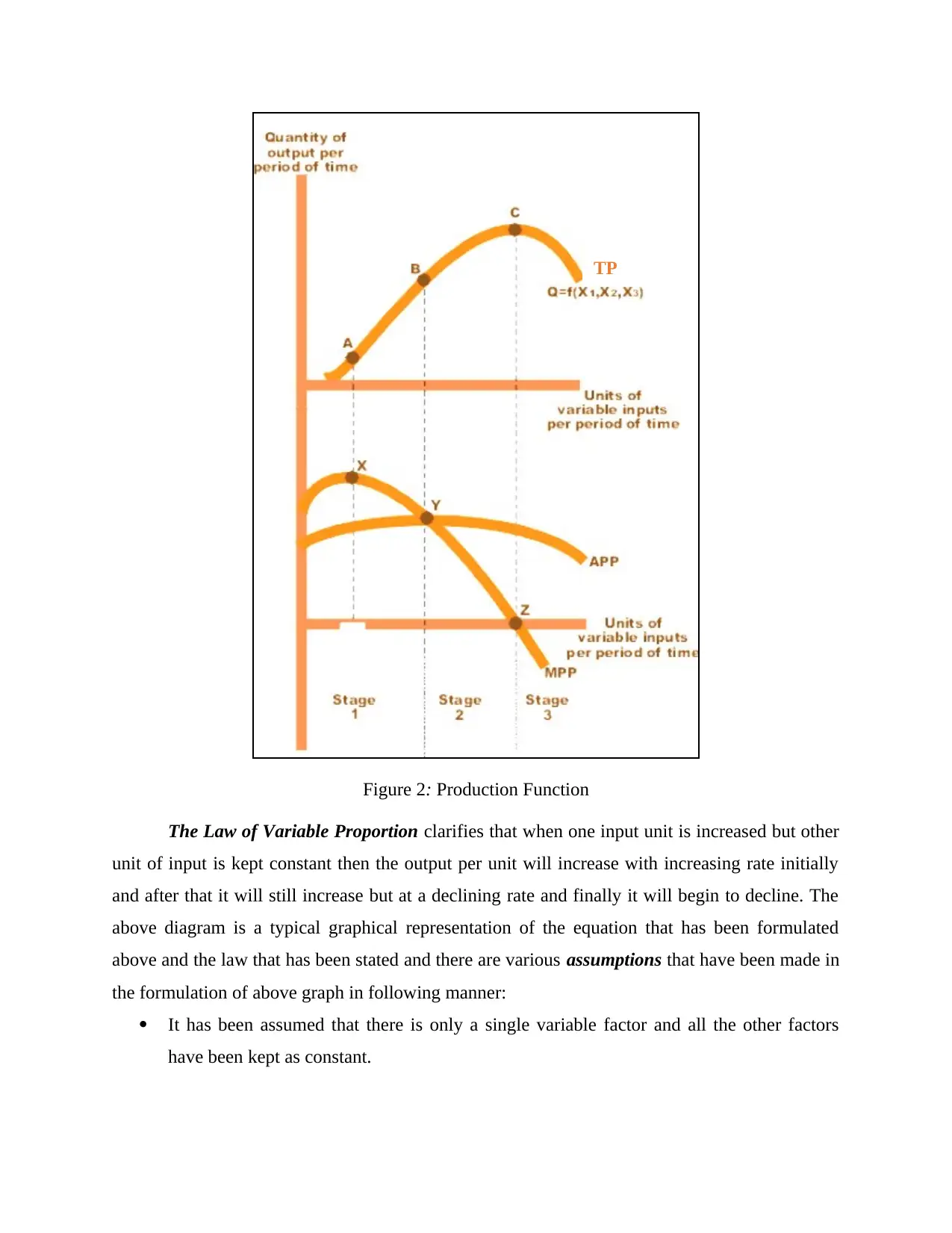
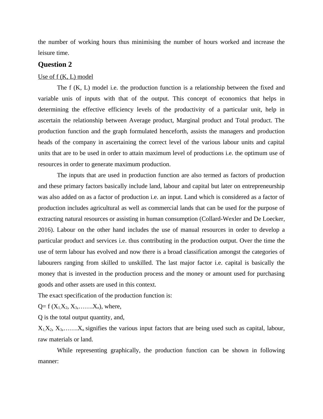
Figure 2: Production Function
The Law of Variable Proportion clarifies that when one input unit is increased but other
unit of input is kept constant then the output per unit will increase with increasing rate initially
and after that it will still increase but at a declining rate and finally it will begin to decline. The
above diagram is a typical graphical representation of the equation that has been formulated
above and the law that has been stated and there are various assumptions that have been made in
the formulation of above graph in following manner:
It has been assumed that there is only a single variable factor and all the other factors
have been kept as constant.
TP
Paraphrase This Document
Need a fresh take? Get an instant paraphrase of this document with our AI Paraphraser
The proportions in which the various input factors have been combined together can be
changed any time.
All the variable factors are categorised as homogenous.
The price of the product and technology remains constant.
There is a short-run situation and the end product is measured in measurable units in
physical terms i.e. tonnes, quintals etc.
In assistance with the graph above, an additional table can be used to understand the various
stages that have been depicted in the graph that has been drawn to represent the production
function (Kennedy, 2017). The following table helps in understanding that at different stages
what is the input level and how much output can be generated from such input levels:
Figure 3: Schedule of Input and Output
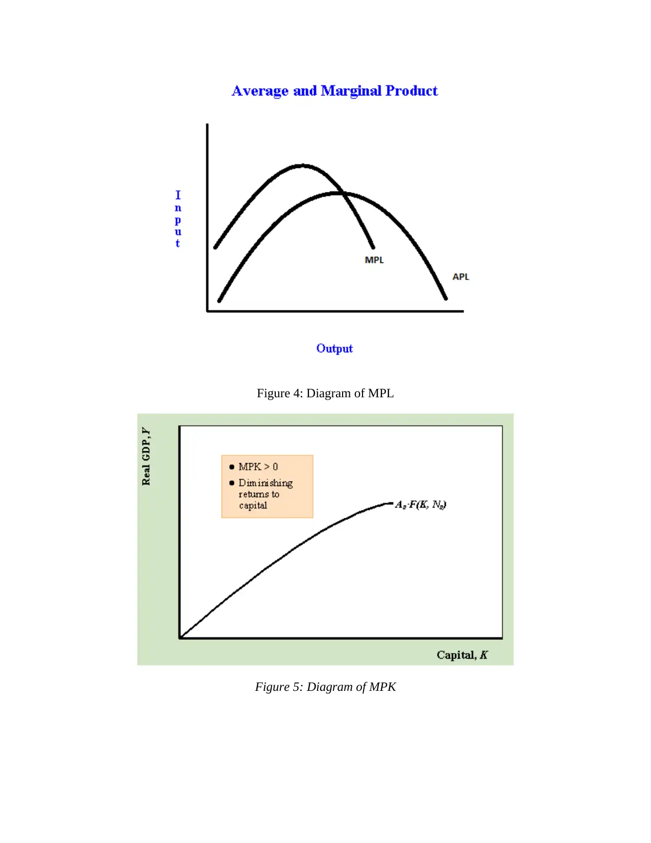
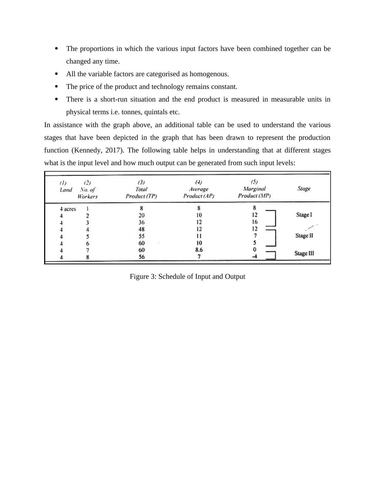
Figure 4: Diagram of MPL
Figure 5: Diagram of MPK
Figure 5: Diagram of MPK
⊘ This is a preview!⊘
Do you want full access?
Subscribe today to unlock all pages.
Trusted by 1+ million students worldwide
When the above table is linked with the production function graph, it can be ascertained
that based on the units of labour input with the land units remaining constant, there are three
broad categories that have emerged:
Stage 1: When the total number of workers or labourers is being increased at a constant
rate, initially the Marginal Product will increase at increasing rate due to the total product
and the average product increasing steadily.
Stage 2: This arises when the Total Product is still increasing with the increase in
labourer’s unit, yet the average product initially becomes constant and then declines thus
resulting in decline of the Marginal Product.
Stage 3: This arises when the total product after becoming constant, begins to decline and
the average product too declines but at a lower rate than Marginal Product.
For a firm, the best strategy is to select the appropriate units of input in terms of labour and
capital based on the time run, i.e. in the short run, the company cannot shift the capital that is
being employed and has to bear its cost but it can select the different levels of labourers
employed in the firm and thus try to minimise the cost (Grieco, Li and Zhang, 2016). In longer
run, the company can change the level of capital as well as labour employed so as to manage the
return levels of the inputs employed.
Question 3
Consumption of Tea
An inferior good can be termed as that good whose consumption decreases when the
income level of the consumers’ increases and normal good on the other hand is termed as that
good whose consumption increases with the increase in income level. In the current question
information regarding the consumption pattern of Ann in respect to Tea has been given and it has
been stated that as the prices of tea goes down, the consumption of tea increases (Berry and
et.al., 2018). Although, if the consumable income had been given of Ann, it would have ben
easier, but still using the current information given, it can be clearly stated that the goods i.e. Tea
is Normal Good. The income and substitution effect states that amongst two substitute goods X
and Y, if the price of good X decreases, then he will automatically buy more of Good X and
reduce the good Y.
Paraphrase This Document
Need a fresh take? Get an instant paraphrase of this document with our AI Paraphraser
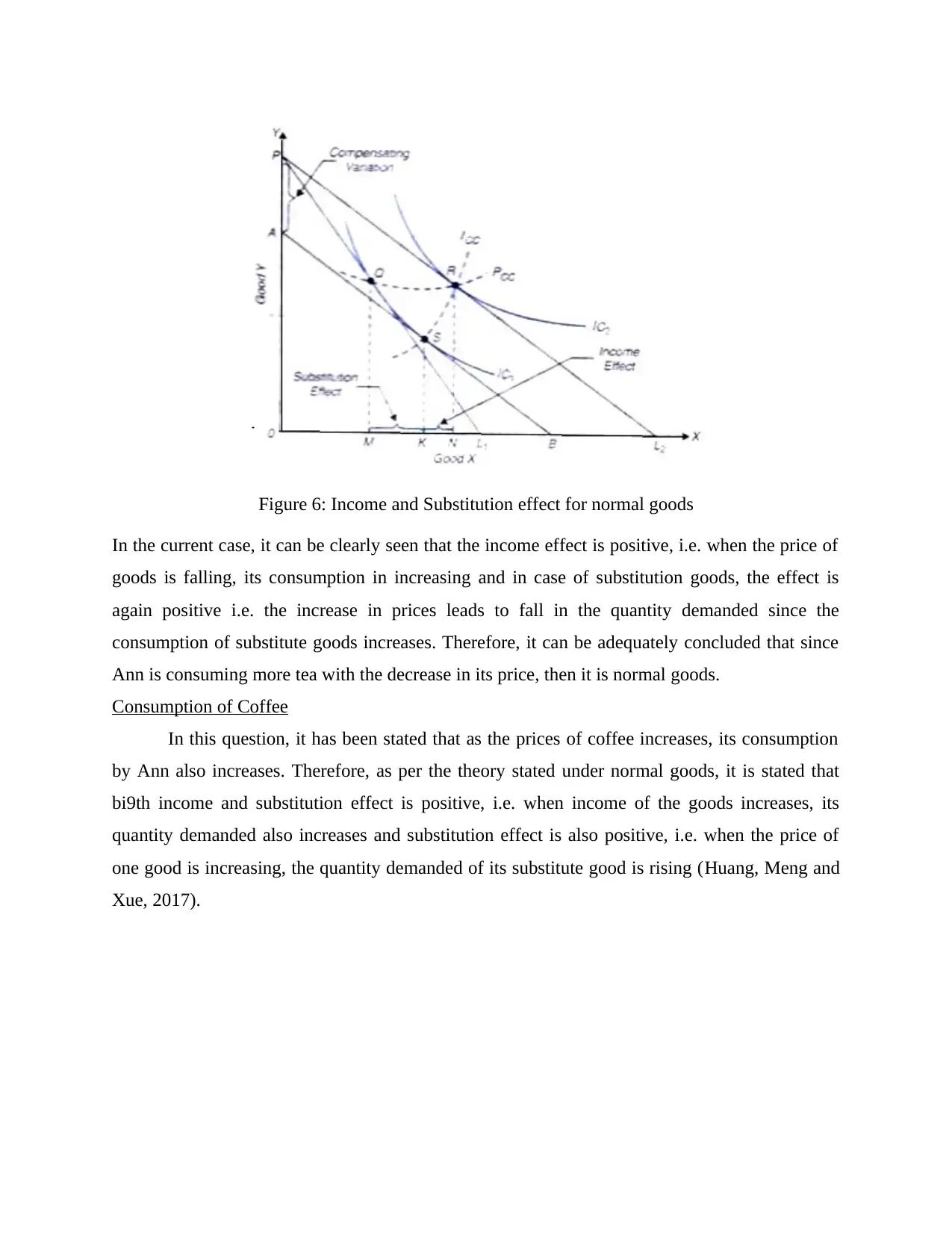
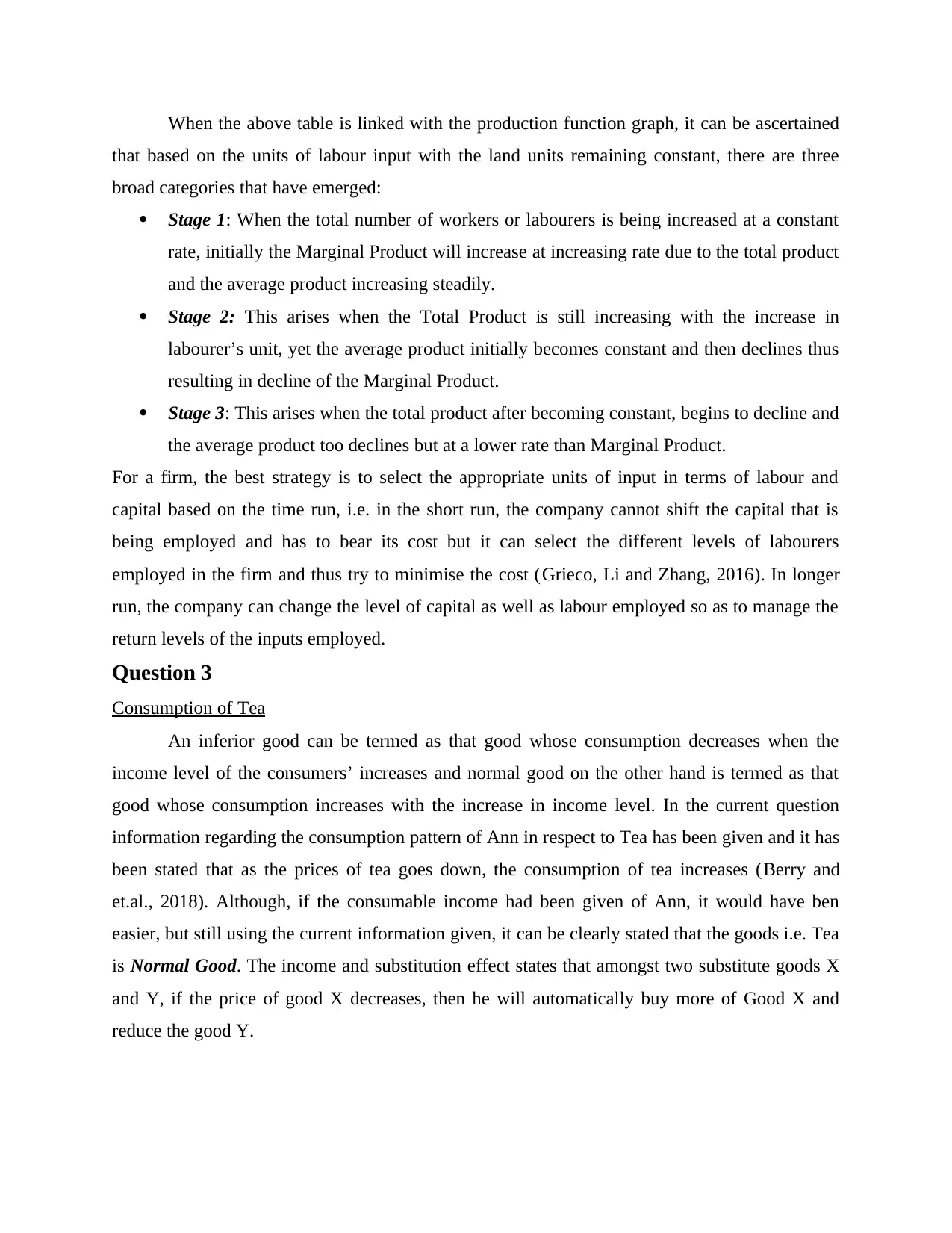
Figure 6: Income and Substitution effect for normal goods
In the current case, it can be clearly seen that the income effect is positive, i.e. when the price of
goods is falling, its consumption in increasing and in case of substitution goods, the effect is
again positive i.e. the increase in prices leads to fall in the quantity demanded since the
consumption of substitute goods increases. Therefore, it can be adequately concluded that since
Ann is consuming more tea with the decrease in its price, then it is normal goods.
Consumption of Coffee
In this question, it has been stated that as the prices of coffee increases, its consumption
by Ann also increases. Therefore, as per the theory stated under normal goods, it is stated that
bi9th income and substitution effect is positive, i.e. when income of the goods increases, its
quantity demanded also increases and substitution effect is also positive, i.e. when the price of
one good is increasing, the quantity demanded of its substitute good is rising (Huang, Meng and
Xue, 2017).
Figure 7: Income and Substitution Effect
In the current case, it can be clearly seen that with increase in the price of coffee, the
consumption of it by Ann is continuously rising and therefore this shows that despite having
other substitute options, Ann is not compromising with or reducing the consumption of coffee
thus showing that these goods are normal or further it can be concluded that these goods are
more than normal i.e. superior goods. Therefore, in accordance with the increase in consumption
with the increase in prices can be termed as the nature of normal goods and therefore, as per the
rule of income and substitution effect along with the increasing consumption helps in effectively
concluding that the coffee is a normal good for Ann.
CONCLUSION
The research carried in the above report can help in concluding that the various concepts
that have been discussed in the report were each useful in analysing different requirements of the
report. The leisure and consumption time of Ann was analysed and appropriate Budget constraint
was developed as per hour wage rate and working hours. Further the report identified the concept
of Production function and finally, the income substitution effect of tea and coffee was analysed
and adequately determined in order to analyse the consumption of Tea and Coffee of Ann and
categorise it into normal or inferior goods.
⊘ This is a preview!⊘
Do you want full access?
Subscribe today to unlock all pages.
Trusted by 1+ million students worldwide
1 out of 14
Related Documents


Your All-in-One AI-Powered Toolkit for Academic Success.
+13062052269
info@desklib.com
Available 24*7 on WhatsApp / Email
![[object Object]](/_next/static/media/star-bottom.7253800d.svg)
Unlock your academic potential
Copyright © 2020–2026 A2Z Services. All Rights Reserved. Developed and managed by ZUCOL.