Analysis of Laminar and Turbulent Pipe Flow (ENG 590)
VerifiedAdded on 2022/08/10
|19
|3534
|172
Report
AI Summary
This report details an experiment investigating laminar and turbulent pipe flow. The study aimed to examine the differences between these two flow regimes, focusing on concepts like the Reynolds number, head loss, and friction factors. The experimental setup involved a narrow bore tube, a water control valve, and mercury/water manometers to measure head loss. The method included varying the flow rate and observing the flow regime using dye injection. Data collected included head loss, volumetric flow rate, and temperature. Results were presented in tables and graphs, including calculations of Reynolds number, Darcy friction factor, and Blasius friction factor. The report provides a detailed analysis of the data, including error analysis and a comparison of different friction factor calculation methods, concluding with a discussion of the results and their implications in fluid mechanics.
1
Student
Instructor
Title
LAMINAR AND TURBULENT PIPE FLOW.
Date
Student
Instructor
Title
LAMINAR AND TURBULENT PIPE FLOW.
Date
Paraphrase This Document
Need a fresh take? Get an instant paraphrase of this document with our AI Paraphraser
2
Table of Contents
LIST OF FIGURE.....................................................................................................................................2
LIST OF TABLES.....................................................................................................................................2
1: INTRODUCTION.......................................................................................................................................3
2: METHOD..................................................................................................................................................6
3: RESULTS..................................................................................................................................................9
5: DISCUSSION..........................................................................................................................................17
6: CONCLUSION.........................................................................................................................................18
7: BIBLIOGRAPHY......................................................................................................................................19
LIST OF FIGURE
Figure 1: Moody Chart................................................................................................................................5
Figure 2: Water Control Valve....................................................................................................................6
Figure 3: Mercury/Water based Barometer.................................................................................................6
Figure 4: Barometer Interchange switch......................................................................................................7
Figure 5: Mercury Thermometer.................................................................................................................7
Figure 6: Stop watch and Collecting calibrated jar......................................................................................8
Figure 7: Complete Set-up of the experiment..............................................................................................8
Figure 8: The graph of head loss against Volumetric flow rate.................................................................15
Figure 9: The graph of Reynold number against darcy, Blasius and Moody friction factor.......................16
Figure 10: Darcy and Blasius friction factor...............................................................................................17
LIST OF TABLES
Table 1: Pipe Specifications........................................................................................................................9
Table 2: Viscosity and density of water at different temperatures...............................................................9
Table 3: Measured quantities of the experiment..........................................................................................9
Table 4: Derived quantities of the experiment...........................................................................................12
Table 5: Error analysis in volumetric and Average velocity........................................................................13
Table 6: Error analysis in Reynolds number and Darcy friction factor.......................................................14
Table 7: Blasius friction factor...................................................................................................................14
3
LAMINAR AND TURBULENT PIPE FLOW
1: INTRODUCTION
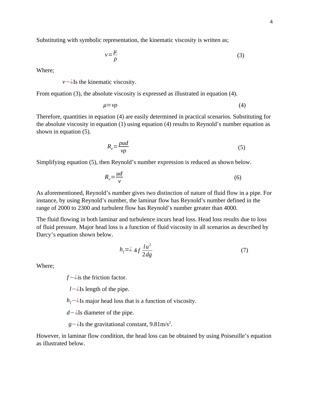
According to fluid mechanics, the flow of the liquid is classified into three categories namely;
laminar flow, transitional flow and turbulent flow. Laminar flow entails the flow of fluid
characterized by smooth streamline and highly ordered flow whereas turbulent flow displays
fluctuation in velocities and highly disordered flow (Www-mdp.eng.cam.ac.uk, 2005). The fluid
flow in laminar flow forms moving layers that are parallel to each other and never crossing at
any point along the flowing channel. Laminar flow can be achieved when the fluid flows at
lower velocity through a smooth pipe with narrow diameter. The counterpart of laminar flow,
turbulent flow, is characterized by moving fluid layers that cross each other along the flowing
channel. The disorderly flow is mainly caused when the fluid is flowing at a high speed or/and in
a pipe whose diameter is relatively large (Mechanical Booster, 2016). Reynold’s number is an
important tool used to distinguish lamina and turbulent flows as well as the transition between
the flows. Reynold’s number, mainly denoted as Re, is basically the ratio resulting from the
inertia forces to viscous forces. The expression of Reynold’s number is as shown in the equation
below.
Re= ρud
μ (1)
Where;
μ−¿Represents the absolute viscosity coefficient in kg/m.s
ρ−¿Represents the mass density in kg/m3.
u−¿Represents the average velocity of the fluid in m/s.
d−¿Represents the diameter of the pipe d (m) that defines characteristic dimension of
fluid flow
Viscosity in fluid mechanics is very fundamental when studying the nature of fluid flow.
Viscosity is the fluid is the inbuilt attributes that offers resistance to flow of fluid. Different
fluids have different viscosities that are dependent on shearing stress between molecules of the
fluid in motion as well as molecules of the flowing fluid in interaction with the walls of the
container in contact. There are two types of viscosity namely; dynamic viscosity and absolute
viscosity. Dynamic viscosity is sometime referred to as absolute viscosity as used in equation
(1). The other type of the viscosity, kinematic viscosity, is expressed as the ratio of mass density
to dynamic viscosity as shown in the equation below.
v= Dynamic∨absolute viscosity
Mass desbsity of the fluid (2)
LAMINAR AND TURBULENT PIPE FLOW
1: INTRODUCTION
According to fluid mechanics, the flow of the liquid is classified into three categories namely;
laminar flow, transitional flow and turbulent flow. Laminar flow entails the flow of fluid
characterized by smooth streamline and highly ordered flow whereas turbulent flow displays
fluctuation in velocities and highly disordered flow (Www-mdp.eng.cam.ac.uk, 2005). The fluid
flow in laminar flow forms moving layers that are parallel to each other and never crossing at
any point along the flowing channel. Laminar flow can be achieved when the fluid flows at
lower velocity through a smooth pipe with narrow diameter. The counterpart of laminar flow,
turbulent flow, is characterized by moving fluid layers that cross each other along the flowing
channel. The disorderly flow is mainly caused when the fluid is flowing at a high speed or/and in
a pipe whose diameter is relatively large (Mechanical Booster, 2016). Reynold’s number is an
important tool used to distinguish lamina and turbulent flows as well as the transition between
the flows. Reynold’s number, mainly denoted as Re, is basically the ratio resulting from the
inertia forces to viscous forces. The expression of Reynold’s number is as shown in the equation
below.
Re= ρud
μ (1)
Where;
μ−¿Represents the absolute viscosity coefficient in kg/m.s
ρ−¿Represents the mass density in kg/m3.
u−¿Represents the average velocity of the fluid in m/s.
d−¿Represents the diameter of the pipe d (m) that defines characteristic dimension of
fluid flow
Viscosity in fluid mechanics is very fundamental when studying the nature of fluid flow.
Viscosity is the fluid is the inbuilt attributes that offers resistance to flow of fluid. Different
fluids have different viscosities that are dependent on shearing stress between molecules of the
fluid in motion as well as molecules of the flowing fluid in interaction with the walls of the
container in contact. There are two types of viscosity namely; dynamic viscosity and absolute
viscosity. Dynamic viscosity is sometime referred to as absolute viscosity as used in equation
(1). The other type of the viscosity, kinematic viscosity, is expressed as the ratio of mass density
to dynamic viscosity as shown in the equation below.
v= Dynamic∨absolute viscosity
Mass desbsity of the fluid (2)
⊘ This is a preview!⊘
Do you want full access?
Subscribe today to unlock all pages.
Trusted by 1+ million students worldwide
4
Substituting with symbolic representation, the kinematic viscosity is written as;
v= μ
ρ (3)
Where;
v−¿Is the kinematic viscosity.
From equation (3), the absolute viscosity is expressed as illustrated in equation (4).
μ=vρ (4)
Therefore, quantities in equation (4) are easily determined in practical scenarios. Substituting for
the absolute viscosity in equation (1) using equation (4) results to Reynold’s number equation as
shown in equation (5).
Re= ρud
vρ (5)
Simplifying equation (5), then Reynold’s number expression is reduced as shown below.
Re= ud
v (6)
As aforementioned, Reynold’s number gives two distinction of nature of fluid flow in a pipe. For
instance, by using Reynold’s number, the laminar flow has Reynold’s number defined in the
range of 2000 to 2300 and turbulent flow has Reynold’s number greater than 4000.
The fluid flowing in both laminar and turbulence incurs head loss. Head loss results due to loss
of fluid pressure. Major head loss is a function of fluid viscosity in all scenarios as described by
Darcy’s equation shown below.
hf =¿ 4 f lu2
2dg (7)
Where;
f −¿is the friction factor.
l−¿Is length of the pipe.
hf −¿Is major head loss that is a function of viscosity.
d−¿Is diameter of the pipe.
g−¿Is the gravitational constant, 9.81m/s2.
However, in laminar flow condition, the head loss can be obtained by using Poiseuille’s equation
as illustrated below.
Paraphrase This Document
Need a fresh take? Get an instant paraphrase of this document with our AI Paraphraser
5
hf =128 vl
πg d4 ˙V (8)
Where;
g−¿is the gravitational acceleration constant.
˙V −¿ ¿Is the volumetric flow rate of the fluid
The graph of head loss against volumetric flow rate in the lamina flow region is a characterized
by a straight line emanating from the origin and whose slope is equivalent to the magnitude of
the expression shown below.
Slope=128 vl
πg d4 (9)
Friction factor is the property of the fluid that is dependent on the shear stress and kinetic energy
possessed by the fluid. As analyzed from equation (7), the friction factor is among the
parameters that directly affects head loss of the flowing fluids. When flow of the fluid is laminar,
the friction factor is given by the expression (Fsl.orst.edu, 2020);
f = 16
Re
(10)
For the turbulent flow region, given that the channel surface of the pipe is smooth, the friction
factor valid for Reynold’s number in the range of 4000< ℜ<1 05 , is given by the Blasius’
equation as shown below.
f = 0.079
ℜ0.25 (11)
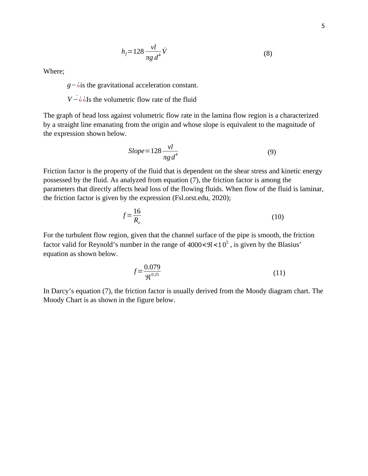
In Darcy’s equation (7), the friction factor is usually derived from the Moody diagram chart. The
Moody Chart is as shown in the figure below.
hf =128 vl
πg d4 ˙V (8)
Where;
g−¿is the gravitational acceleration constant.
˙V −¿ ¿Is the volumetric flow rate of the fluid
The graph of head loss against volumetric flow rate in the lamina flow region is a characterized
by a straight line emanating from the origin and whose slope is equivalent to the magnitude of
the expression shown below.
Slope=128 vl
πg d4 (9)
Friction factor is the property of the fluid that is dependent on the shear stress and kinetic energy
possessed by the fluid. As analyzed from equation (7), the friction factor is among the
parameters that directly affects head loss of the flowing fluids. When flow of the fluid is laminar,
the friction factor is given by the expression (Fsl.orst.edu, 2020);
f = 16
Re
(10)
For the turbulent flow region, given that the channel surface of the pipe is smooth, the friction
factor valid for Reynold’s number in the range of 4000< ℜ<1 05 , is given by the Blasius’
equation as shown below.
f = 0.079
ℜ0.25 (11)
In Darcy’s equation (7), the friction factor is usually derived from the Moody diagram chart. The
Moody Chart is as shown in the figure below.
6
Figure 1: Moody Chart
This chart consists of a family of curves whose shapes depend on Darcy’s friction factor,
roughness of the pipe’s surface of a given diameter and Reynold’s number.
2: METHOD
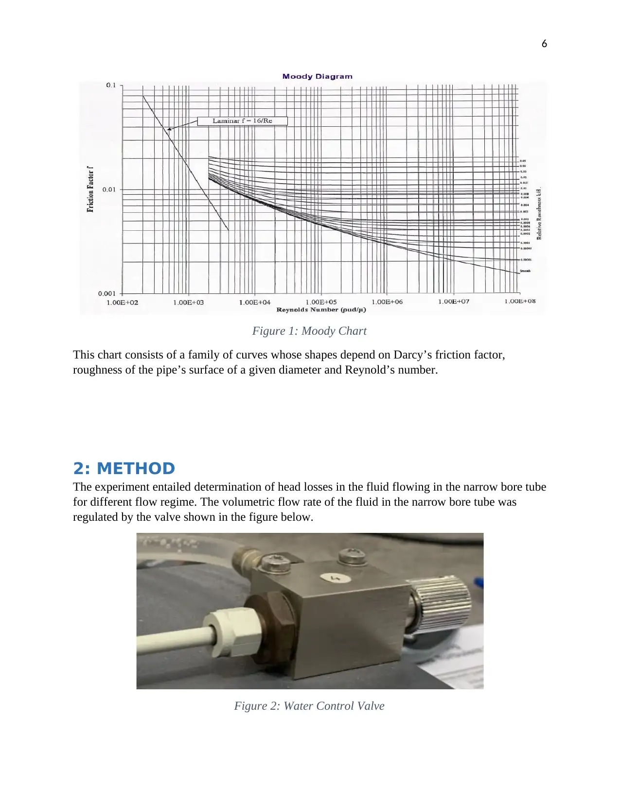
The experiment entailed determination of head losses in the fluid flowing in the narrow bore tube
for different flow regime. The volumetric flow rate of the fluid in the narrow bore tube was
regulated by the valve shown in the figure below.
Figure 2: Water Control Valve
Figure 1: Moody Chart
This chart consists of a family of curves whose shapes depend on Darcy’s friction factor,
roughness of the pipe’s surface of a given diameter and Reynold’s number.
2: METHOD
The experiment entailed determination of head losses in the fluid flowing in the narrow bore tube
for different flow regime. The volumetric flow rate of the fluid in the narrow bore tube was
regulated by the valve shown in the figure below.
Figure 2: Water Control Valve
⊘ This is a preview!⊘
Do you want full access?
Subscribe today to unlock all pages.
Trusted by 1+ million students worldwide
7
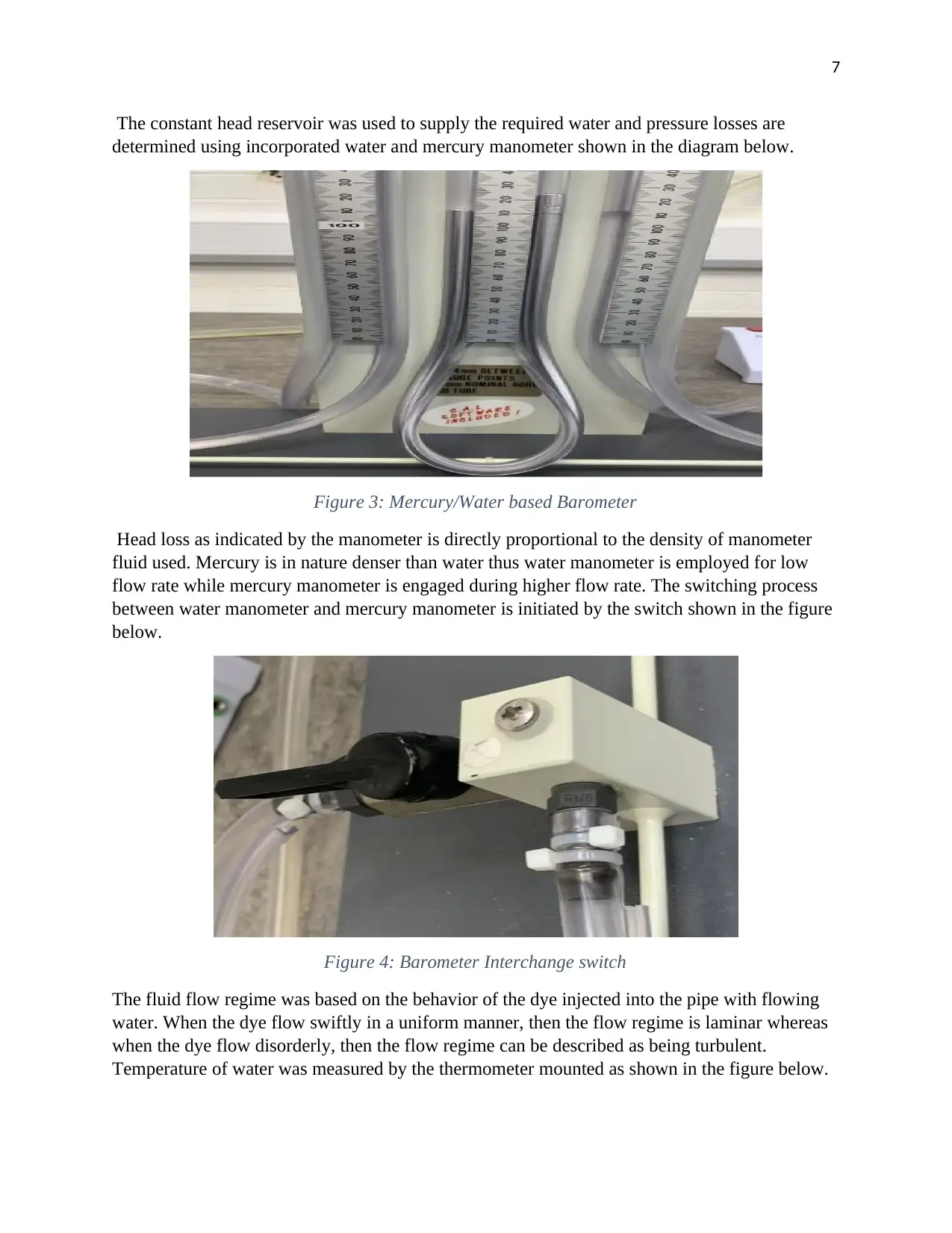
The constant head reservoir was used to supply the required water and pressure losses are
determined using incorporated water and mercury manometer shown in the diagram below.
Figure 3: Mercury/Water based Barometer
Head loss as indicated by the manometer is directly proportional to the density of manometer
fluid used. Mercury is in nature denser than water thus water manometer is employed for low
flow rate while mercury manometer is engaged during higher flow rate. The switching process
between water manometer and mercury manometer is initiated by the switch shown in the figure
below.
Figure 4: Barometer Interchange switch
The fluid flow regime was based on the behavior of the dye injected into the pipe with flowing
water. When the dye flow swiftly in a uniform manner, then the flow regime is laminar whereas
when the dye flow disorderly, then the flow regime can be described as being turbulent.
Temperature of water was measured by the thermometer mounted as shown in the figure below.
Paraphrase This Document
Need a fresh take? Get an instant paraphrase of this document with our AI Paraphraser
8
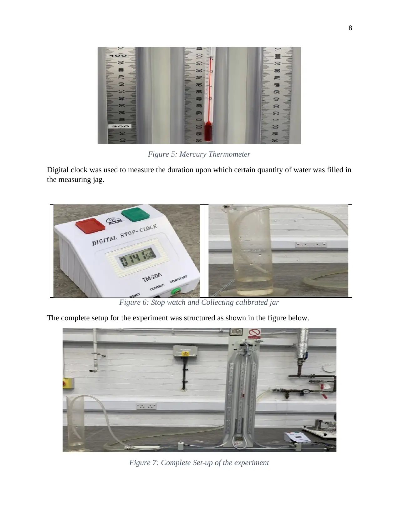
Figure 5: Mercury Thermometer
Digital clock was used to measure the duration upon which certain quantity of water was filled in
the measuring jag.
Figure 6: Stop watch and Collecting calibrated jar
The complete setup for the experiment was structured as shown in the figure below.
Figure 7: Complete Set-up of the experiment
9
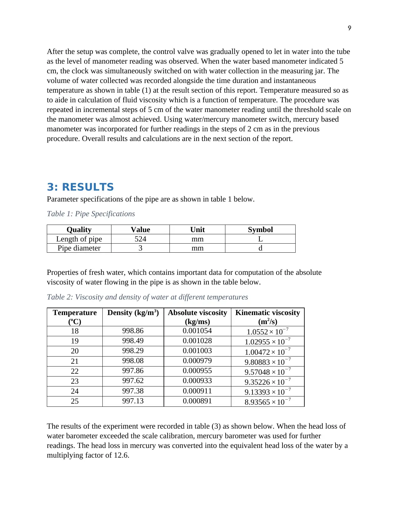
After the setup was complete, the control valve was gradually opened to let in water into the tube
as the level of manometer reading was observed. When the water based manometer indicated 5
cm, the clock was simultaneously switched on with water collection in the measuring jar. The
volume of water collected was recorded alongside the time duration and instantaneous
temperature as shown in table (1) at the result section of this report. Temperature measured so as
to aide in calculation of fluid viscosity which is a function of temperature. The procedure was
repeated in incremental steps of 5 cm of the water manometer reading until the threshold scale on
the manometer was almost achieved. Using water/mercury manometer switch, mercury based
manometer was incorporated for further readings in the steps of 2 cm as in the previous
procedure. Overall results and calculations are in the next section of the report.
3: RESULTS
Parameter specifications of the pipe are as shown in table 1 below.
Table 1: Pipe Specifications
Quality Value Unit Symbol
Length of pipe 524 mm L
Pipe diameter 3 mm d
Properties of fresh water, which contains important data for computation of the absolute
viscosity of water flowing in the pipe is as shown in the table below.
Table 2: Viscosity and density of water at different temperatures
Temperature
(oC)
Density (kg/m3) Absolute viscosity
(kg/ms)
Kinematic viscosity
(m2/s)
18 998.86 0.001054 1.0552× 10⁻⁷
19 998.49 0.001028 1.02955 ×10⁻⁷
20 998.29 0.001003 1.00472× 10⁻⁷
21 998.08 0.000979 9.80883 ×10⁻⁷
22 997.86 0.000955 9.57048 ×10⁻⁷
23 997.62 0.000933 9.35226 ×10⁻⁷
24 997.38 0.000911 9.13393 ×10⁻⁷
25 997.13 0.000891 8.93565 ×10⁻⁷
The results of the experiment were recorded in table (3) as shown below. When the head loss of
water barometer exceeded the scale calibration, mercury barometer was used for further
readings. The head loss in mercury was converted into the equivalent head loss of the water by a
multiplying factor of 12.6.
⊘ This is a preview!⊘
Do you want full access?
Subscribe today to unlock all pages.
Trusted by 1+ million students worldwide
10
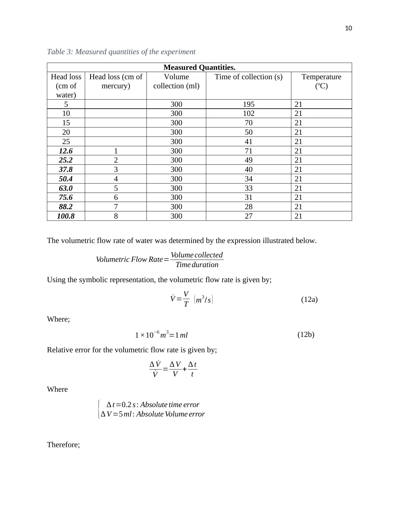
Table 3: Measured quantities of the experiment
Measured Quantities.
Head loss
(cm of
water)
Head loss (cm of
mercury)
Volume
collection (ml)
Time of collection (s) Temperature
(oC)
5 300 195 21
10 300 102 21
15 300 70 21
20 300 50 21
25 300 41 21
12.6 1 300 71 21
25.2 2 300 49 21
37.8 3 300 40 21
50.4 4 300 34 21
63.0 5 300 33 21
75.6 6 300 31 21
88.2 7 300 28 21
100.8 8 300 27 21
The volumetric flow rate of water was determined by the expression illustrated below.
Volumetric Flow Rate= Volume collected
Time duration
Using the symbolic representation, the volumetric flow rate is given by;
˙V = V
T ( m3 /s ) (12a)
Where;
1 ×10⁻⁶ m3=1 ml (12b)
Relative error for the volumetric flow rate is given by;
∆ ˙V
˙V = ∆ V
V + ∆ t
t
Where
{ ∆ t=0.2 s : Absolute time error
∆ V =5 ml : Absolute Volume error
Therefore;
Paraphrase This Document
Need a fresh take? Get an instant paraphrase of this document with our AI Paraphraser
11
˙V = V
T ± ∆ ˙V ( m3 /s )
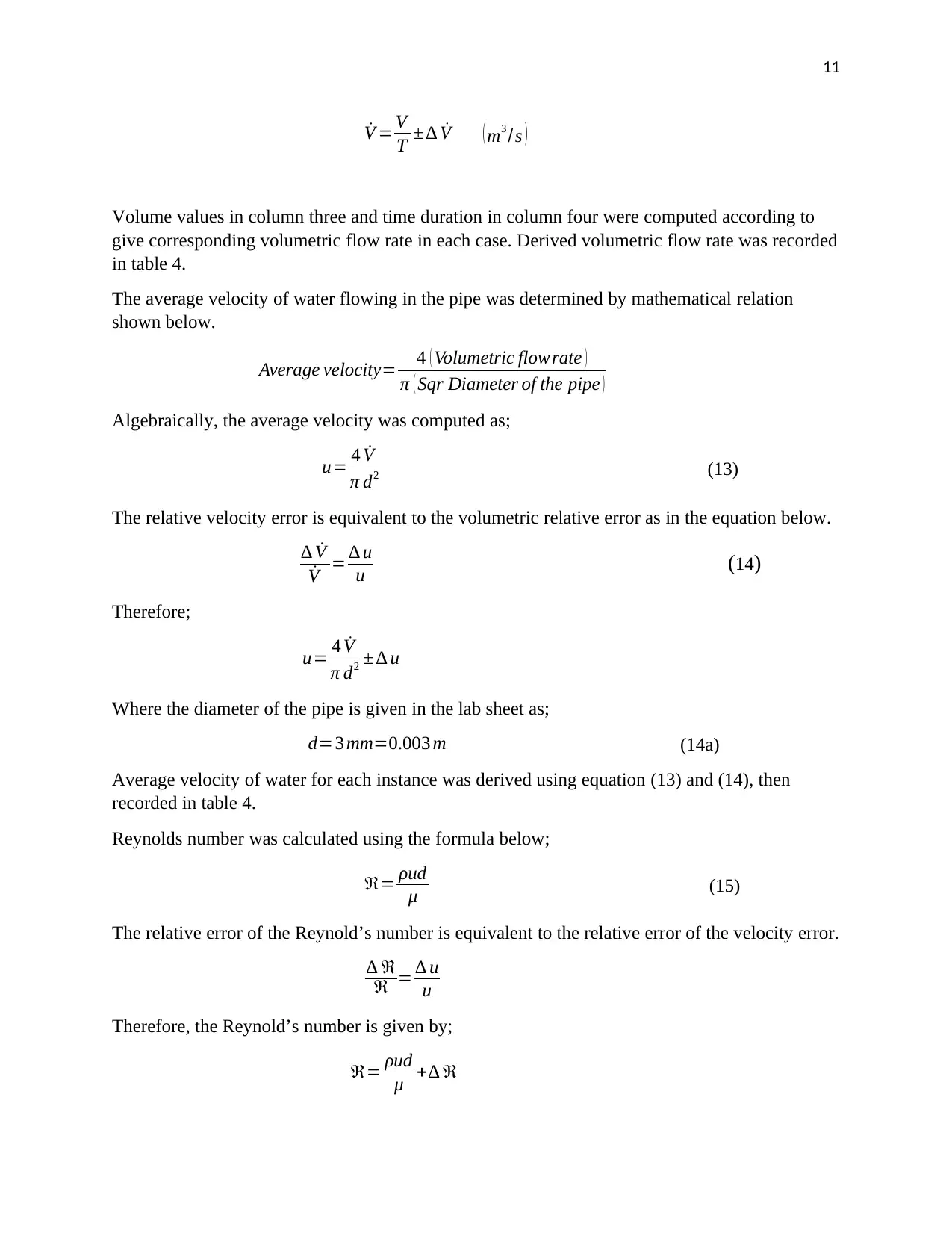
Volume values in column three and time duration in column four were computed according to
give corresponding volumetric flow rate in each case. Derived volumetric flow rate was recorded
in table 4.
The average velocity of water flowing in the pipe was determined by mathematical relation
shown below.
Average velocity= 4 ( Volumetric flowrate )
π ( Sqr Diameter of the pipe )
Algebraically, the average velocity was computed as;
u= 4 ˙V
π d2 (13)
The relative velocity error is equivalent to the volumetric relative error as in the equation below.
∆ ˙V
˙V = ∆ u
u (14)
Therefore;
u= 4 ˙V
π d2 ± ∆ u
Where the diameter of the pipe is given in the lab sheet as;
d=3 mm=0.003 m (14a)
Average velocity of water for each instance was derived using equation (13) and (14), then
recorded in table 4.
Reynolds number was calculated using the formula below;
ℜ= ρud
μ (15)
The relative error of the Reynold’s number is equivalent to the relative error of the velocity error.
∆ ℜ
ℜ = ∆ u
u
Therefore, the Reynold’s number is given by;
ℜ= ρud
μ +∆ ℜ
˙V = V
T ± ∆ ˙V ( m3 /s )
Volume values in column three and time duration in column four were computed according to
give corresponding volumetric flow rate in each case. Derived volumetric flow rate was recorded
in table 4.
The average velocity of water flowing in the pipe was determined by mathematical relation
shown below.
Average velocity= 4 ( Volumetric flowrate )
π ( Sqr Diameter of the pipe )
Algebraically, the average velocity was computed as;
u= 4 ˙V
π d2 (13)
The relative velocity error is equivalent to the volumetric relative error as in the equation below.
∆ ˙V
˙V = ∆ u
u (14)
Therefore;
u= 4 ˙V
π d2 ± ∆ u
Where the diameter of the pipe is given in the lab sheet as;
d=3 mm=0.003 m (14a)
Average velocity of water for each instance was derived using equation (13) and (14), then
recorded in table 4.
Reynolds number was calculated using the formula below;
ℜ= ρud
μ (15)
The relative error of the Reynold’s number is equivalent to the relative error of the velocity error.
∆ ℜ
ℜ = ∆ u
u
Therefore, the Reynold’s number is given by;
ℜ= ρud
μ +∆ ℜ
12
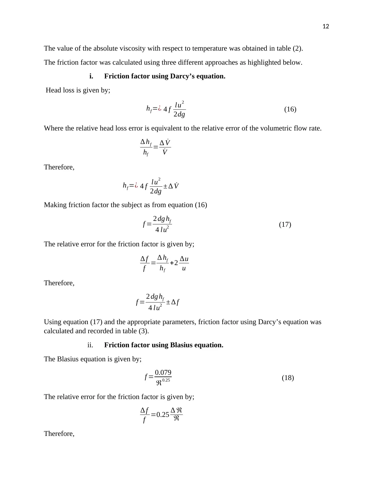
The value of the absolute viscosity with respect to temperature was obtained in table (2).
The friction factor was calculated using three different approaches as highlighted below.
i. Friction factor using Darcy’s equation.
Head loss is given by;
hf =¿ 4 f lu2
2dg (16)
Where the relative head loss error is equivalent to the relative error of the volumetric flow rate.
∆ hf
hf
= ∆ ˙V
˙V
Therefore,
hf =¿ 4 f lu2
2dg ± ∆ ˙V
Making friction factor the subject as from equation (16)
f = 2 dg hf
4 lu2 (17)
The relative error for the friction factor is given by;
∆ f
f = ∆ hf
hf
+2 ∆u
u
Therefore,
f = 2 dg hf
4 l u2 ± ∆ f
Using equation (17) and the appropriate parameters, friction factor using Darcy’s equation was
calculated and recorded in table (3).
ii. Friction factor using Blasius equation.
The Blasius equation is given by;
f = 0.079
ℜ0.25 (18)
The relative error for the friction factor is given by;
∆ f
f =0.25 ∆ ℜ
ℜ
Therefore,
⊘ This is a preview!⊘
Do you want full access?
Subscribe today to unlock all pages.
Trusted by 1+ million students worldwide
1 out of 19
Related Documents


Your All-in-One AI-Powered Toolkit for Academic Success.
+13062052269
info@desklib.com
Available 24*7 on WhatsApp / Email
![[object Object]](/_next/static/media/star-bottom.7253800d.svg)
Unlock your academic potential
Copyright © 2020–2026 A2Z Services. All Rights Reserved. Developed and managed by ZUCOL.