LB5235: SP1 Applied Research Project - SPSS Based Data Analysis

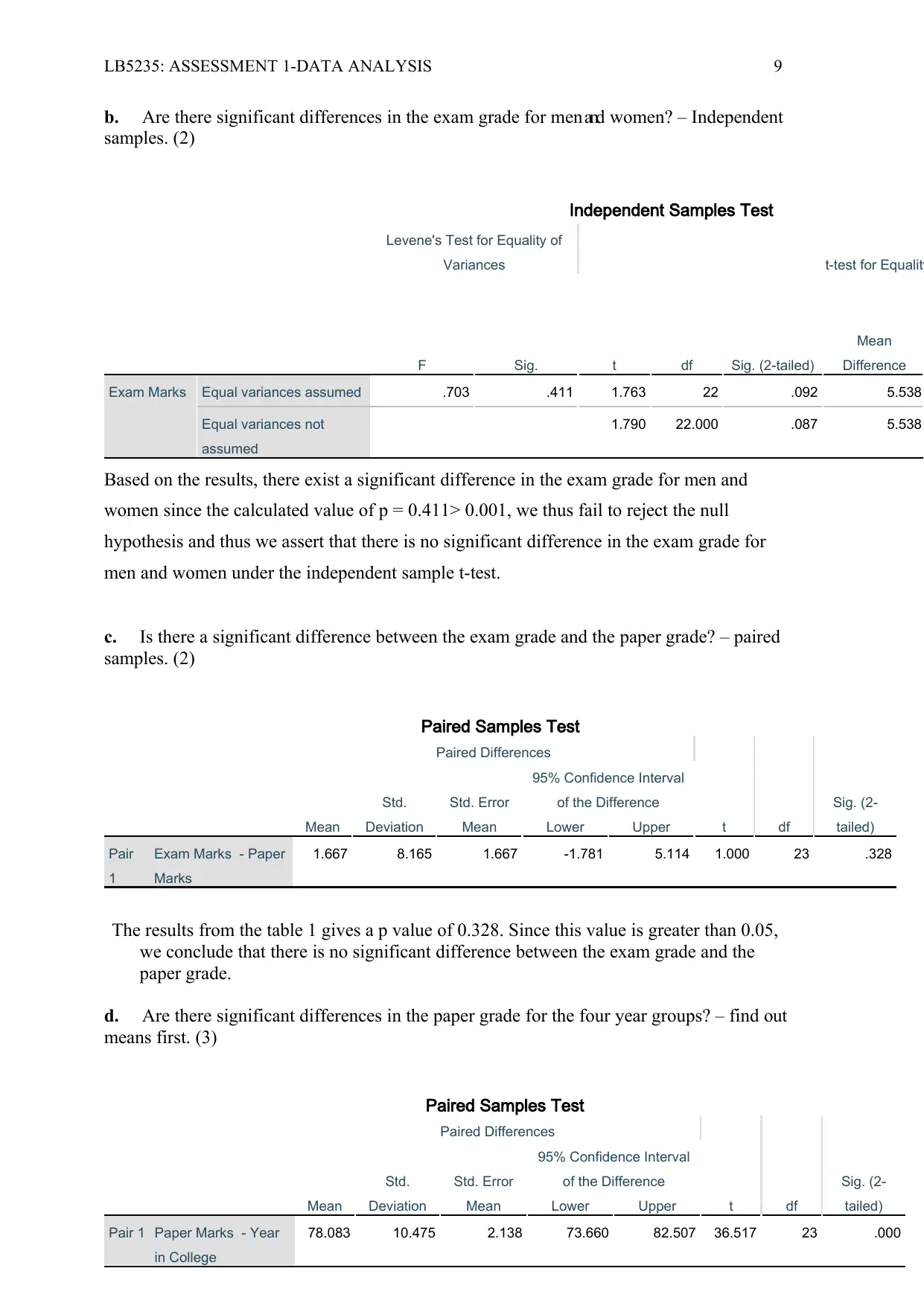
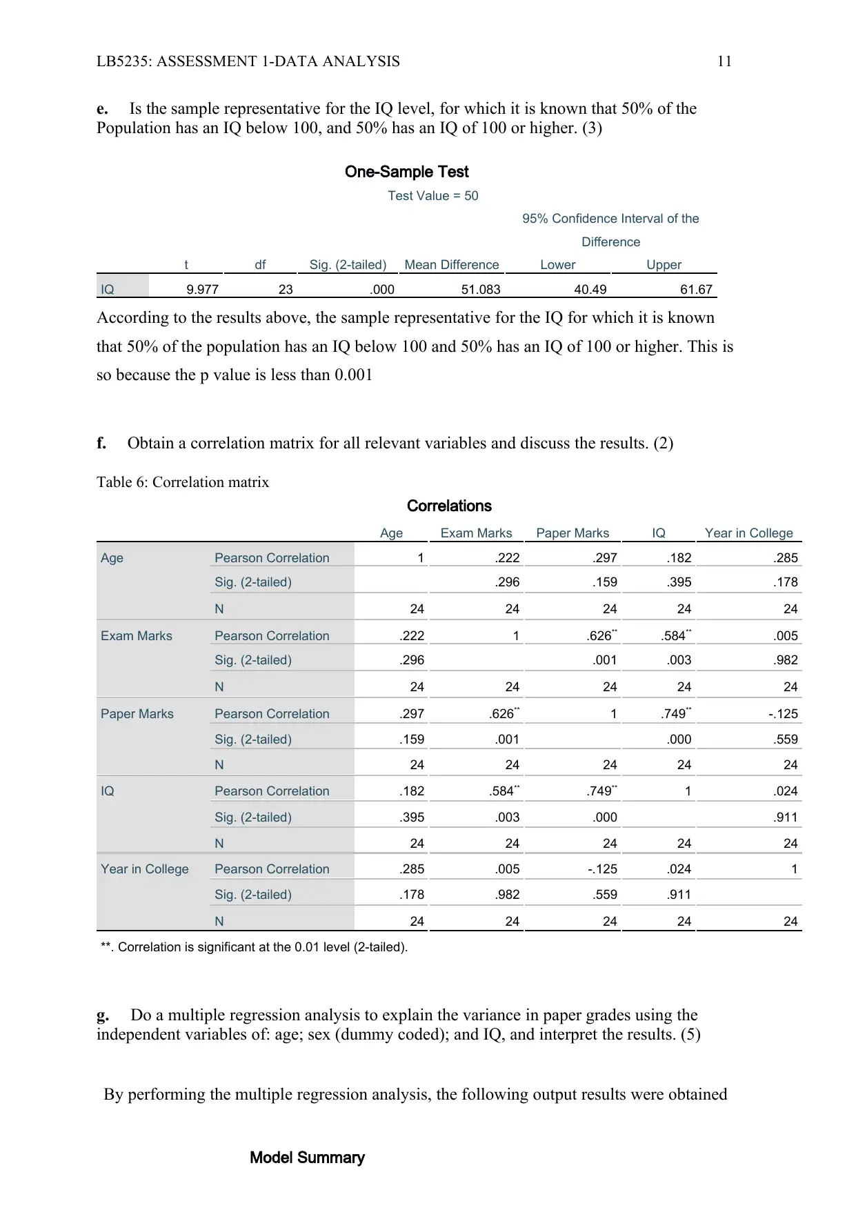
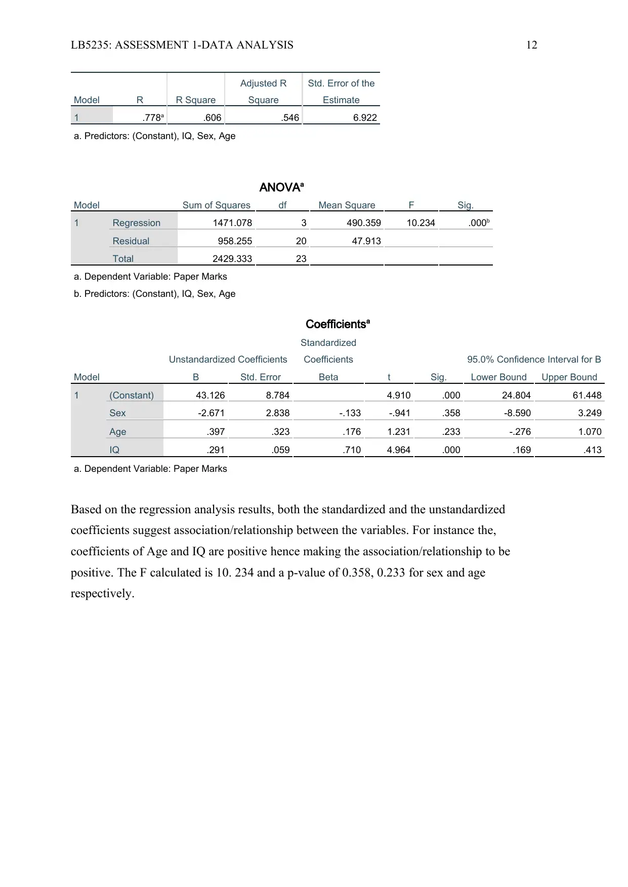
This assignment, likely for the course LB5235 Applied Research Project, showcases data analysis performed using SPSS. The student begins by handling a dataset with variables like age, exam marks, paper marks, sex, year in college, and IQ. Descriptive statistics are generated for metric variables, and non-metric variables are summarized using frequencies and pie charts. Histograms and scatter plots are created to visualize relationships between variables. The analysis includes recoding variables, computing mean IQ for different groups, and creating dummy variables. Furthermore, the assignment delves into data analysis techniques such as t-tests (one-sample, independent samples, and paired samples), correlation matrices, and multiple regression analysis to explore relationships between variables and test hypotheses, interpreting the results in the context of the research project. Part 2 touches on Methodology. The document concludes with references to relevant statistical resources.

Running head: LB5235: ASSESSMENT 1-DATA ANALYSIS 1
LB5235: Assessment 1 – Data Analysis
By (Name of Student
(Institutional Affiliation)
(Date of Submission)

LB5235: ASSESSMENT 1-DATA ANALYSIS 2
1. Data handling
a. Enter the data in the computer. (2 marks)
b. Provide appropriate variable labels, values labels, and scaling indications to the
variables. (2)
Screenshot

LB5235: ASSESSMENT 1-DATA ANALYSIS 3
2. Descriptives
a. Use Analyze, Descriptive statistics, Descriptives to summarize metric variables. (3)
The table 1 below display the descriptive statistics of the metric variables as obtained from
SPSS output window.
Table 1: Summary Statistics for Metric Variables
Descriptive Statistics
N
Minimu
m
Maximu
m Mean
Std.
Deviation
Varianc
e Skewness Kurtosis
Statistic Statistic Statistic Statistic
Std.
Error Statistic Statistic Statistic
Std.
Error Statistic
Std.
Error
Age 24 17 35 22.96 .931 4.563 20.824 1.209 .472 .932 .918
Exam Marks 24 67 97 82.00 1.635 8.011 64.174 -.020 .472 -.568 .918
Paper Marks 24 57 95 80.33 2.098 10.277 105.623 -.669 .472 .108 .918
IQ 24 60 165 101.08 5.120 25.082 629.123 .613 .472 .295 .918

LB5235: ASSESSMENT 1-DATA ANALYSIS 4
Valid N
(listwise)
24
b. Recode the sex variable such that it is 1 for females and 0 for males. Hint: Do this
immediately in your own dataset, so do not enter M and F. (3)
Screenshot
c. Use Analyze, Descriptive statistics, Frequencies to summarize nonmetric variables. (3)
Table 2: Summary Statistics for Sex
Sex
Frequency Percent Valid Percent Cumulative Percent
Valid 0 11 45.8 45.8 45.8
1 13 54.2 54.2 100.0
Total 24 100.0 100.0
Table 3: Summary Statistics for Year in College

LB5235: ASSESSMENT 1-DATA ANALYSIS 5
Year in College
Frequency Percent Valid Percent Cumulative Percent
Valid 1 8 33.3 33.3 33.3
2 6 25.0 25.0 58.3
3 6 25.0 25.0 83.3
4 4 16.7 16.7 100.0
Total 24 100.0 100.0
d. Create a pie-chart for Year in College. (2)
Figure 1: Pie Chart for Year in College
e. Create a histogram for IQ and include the normal distribution. (2)
Figure 2: Histogram for IQ with the normal distribution curve

LB5235: ASSESSMENT 1-DATA ANALYSIS 6
Figure 2: Histogram for IQ with the normal distribution curve
f. Make a scatter plot with IQ on the x-axis and exam grade on the y-axis. What do you
conclude? (3)
Figure 4: Scatter plot of IQ and Exam Grade

LB5235: ASSESSMENT 1-DATA ANALYSIS 7
From the scatter plot above, the data indicates/shows uphill pattern. This suggest that there
exist a positive relationship between exam marks and the IQ. It thus follows that exam marks
increases with an absolute increase in the IQ of the student/individual
g. Make a scatter plot with year in college on the x-axis and IQ on the y-axis. What do you
conclude? (3)
The scatter plot of IQ against year in college as shown above indicates that the data is
normally distributes and there exist no outliers in the data either. The regression line added
in the scatter plot further suggest that there exist some level and the degree of association.
h. Compute the mean IQ for males and for females. Conclusion? (2)
Table 6: Mean IQ for Males and for Females.
Mean IQ
N Mean
Males 12 102.33
Females 12 89.33
Valid N (listwise) 12
From the table above, the mean IQ for males and females are 102.33 and 89.33 respectively.
The average mean for males is higher than that of female. That is 102.33 > 89.33.
i. Create a new dummy variable, IQdum, which is 1 if the IQ is larger than or equal to
100, and 0 else. (3)

LB5235: ASSESSMENT 1-DATA ANALYSIS 8
j. Create a cross table between IQdum and Year in College. (2)
Table 4: Cross table between IQdum and Year in College
IOdum * Year in College Crosstabulation
Count
Year in College
Total1 2 3 4
IOdum .00 4 3 5 2 14
1.00 4 3 1 2 10
Total 8 6 6 4 24
3.
4. Data analysis
a. Is the exam grade significantly larger than 75? (3)
Table 5: One Sample Test
One-Sample Test
Test Value = 75
t df Sig. (2-tailed) Mean Difference
95% Confidence Interval of the Differ
Lower Upper
Exam Marks 4.281 23 .000 7.000 3.62
Based on the results, since p < 0.001, we thus reject the null hypothesis and conclude that the
exam grade significantly larger than 75%.

LB5235: ASSESSMENT 1-DATA ANALYSIS 9
b. Are there significant differences in the exam grade for men and women? – Independent
samples. (2)
Independent Samples Test
Levene's Test for Equality of
Variances t-test for Equality
F Sig. t df Sig. (2-tailed)
Mean
Difference
Exam Marks Equal variances assumed .703 .411 1.763 22 .092 5.538
Equal variances not
assumed
1.790 22.000 .087 5.538
Based on the results, there exist a significant difference in the exam grade for men and
women since the calculated value of p = 0.411> 0.001, we thus fail to reject the null
hypothesis and thus we assert that there is no significant difference in the exam grade for
men and women under the independent sample t-test.
c. Is there a significant difference between the exam grade and the paper grade? – paired
samples. (2)
Paired Samples Test
Paired Differences
t df
Sig. (2-
tailed)Mean
Std.
Deviation
Std. Error
Mean
95% Confidence Interval
of the Difference
Lower Upper
Pair
1
Exam Marks - Paper
Marks
1.667 8.165 1.667 -1.781 5.114 1.000 23 .328
The results from the table 1 gives a p value of 0.328. Since this value is greater than 0.05,
we conclude that there is no significant difference between the exam grade and the
paper grade.
d. Are there significant differences in the paper grade for the four year groups? – find out
means first. (3)
Paired Samples Test
Paired Differences
t df
Sig. (2-
tailed)Mean
Std.
Deviation
Std. Error
Mean
95% Confidence Interval
of the Difference
Lower Upper
Pair 1 Paper Marks - Year
in College
78.083 10.475 2.138 73.660 82.507 36.517 23 .000

LB5235: ASSESSMENT 1-DATA ANALYSIS 10

LB5235: ASSESSMENT 1-DATA ANALYSIS 11
e. Is the sample representative for the IQ level, for which it is known that 50% of the
Population has an IQ below 100, and 50% has an IQ of 100 or higher. (3)
One-Sample Test
Test Value = 50
t df Sig. (2-tailed) Mean Difference
95% Confidence Interval of the
Difference
Lower Upper
IQ 9.977 23 .000 51.083 40.49 61.67
According to the results above, the sample representative for the IQ for which it is known
that 50% of the population has an IQ below 100 and 50% has an IQ of 100 or higher. This is
so because the p value is less than 0.001
f. Obtain a correlation matrix for all relevant variables and discuss the results. (2)
Table 6: Correlation matrix
Correlations
Age Exam Marks Paper Marks IQ Year in College
Age Pearson Correlation 1 .222 .297 .182 .285
Sig. (2-tailed) .296 .159 .395 .178
N 24 24 24 24 24
Exam Marks Pearson Correlation .222 1 .626** .584** .005
Sig. (2-tailed) .296 .001 .003 .982
N 24 24 24 24 24
Paper Marks Pearson Correlation .297 .626** 1 .749** -.125
Sig. (2-tailed) .159 .001 .000 .559
N 24 24 24 24 24
IQ Pearson Correlation .182 .584** .749** 1 .024
Sig. (2-tailed) .395 .003 .000 .911
N 24 24 24 24 24
Year in College Pearson Correlation .285 .005 -.125 .024 1
Sig. (2-tailed) .178 .982 .559 .911
N 24 24 24 24 24
**. Correlation is significant at the 0.01 level (2-tailed).
g. Do a multiple regression analysis to explain the variance in paper grades using the
independent variables of: age; sex (dummy coded); and IQ, and interpret the results. (5)
By performing the multiple regression analysis, the following output results were obtained
Model Summary

LB5235: ASSESSMENT 1-DATA ANALYSIS 12
Model R R Square
Adjusted R
Square
Std. Error of the
Estimate
1 .778a .606 .546 6.922
a. Predictors: (Constant), IQ, Sex, Age
ANOVAa
Model Sum of Squares df Mean Square F Sig.
1 Regression 1471.078 3 490.359 10.234 .000b
Residual 958.255 20 47.913
Total 2429.333 23
a. Dependent Variable: Paper Marks
b. Predictors: (Constant), IQ, Sex, Age
Coefficientsa
Model
Unstandardized Coefficients
Standardized
Coefficients
t Sig.
95.0% Confidence Interval for B
B Std. Error Beta Lower Bound Upper Bound
1 (Constant) 43.126 8.784 4.910 .000 24.804 61.448
Sex -2.671 2.838 -.133 -.941 .358 -8.590 3.249
Age .397 .323 .176 1.231 .233 -.276 1.070
IQ .291 .059 .710 4.964 .000 .169 .413
a. Dependent Variable: Paper Marks
Based on the regression analysis results, both the standardized and the unstandardized
coefficients suggest association/relationship between the variables. For instance the,
coefficients of Age and IQ are positive hence making the association/relationship to be
positive. The F calculated is 10. 234 and a p-value of 0.358, 0.233 for sex and age
respectively.