Advanced Control Theory: Lead-Lag Compensator Design and MATLAB

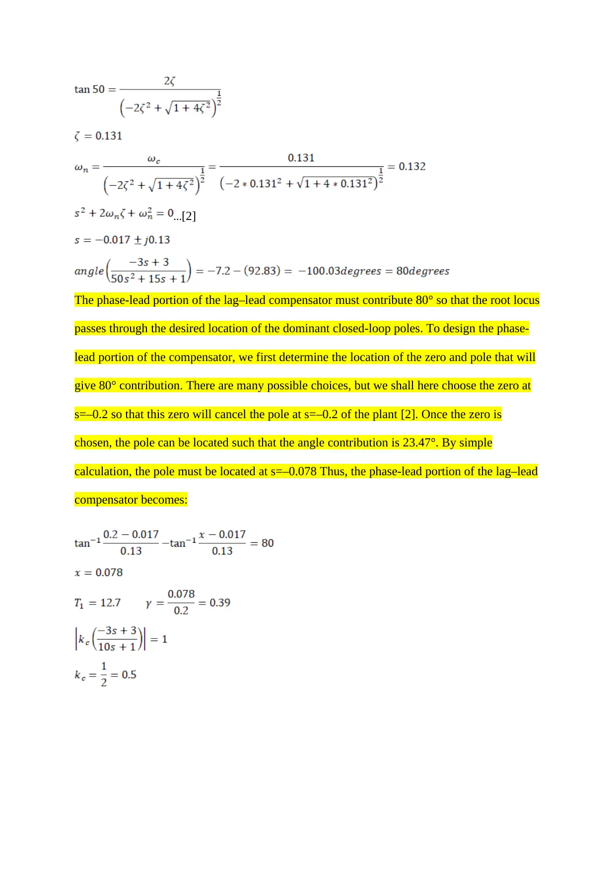
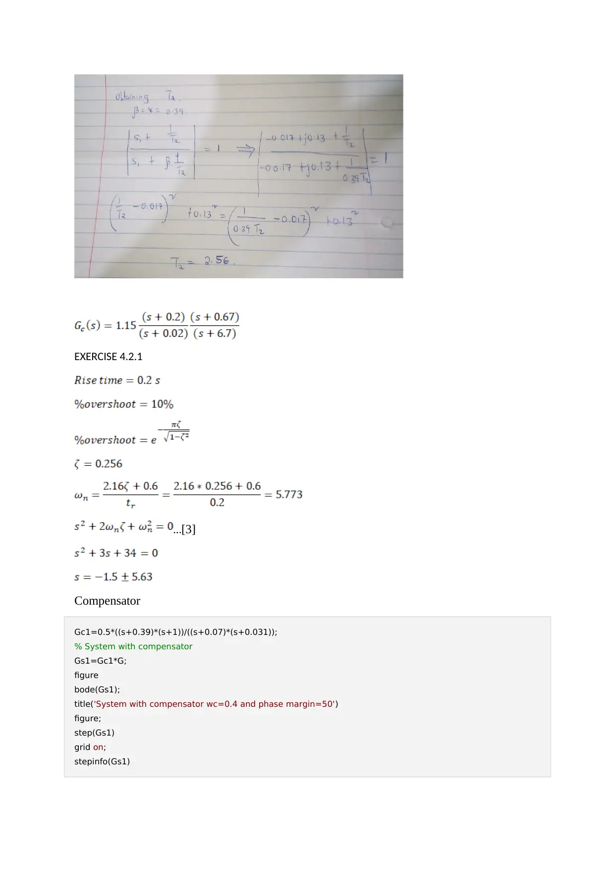
This assignment focuses on the design and analysis of lead-lag compensators within the context of advanced control theory. It includes exercises involving the implementation of lead-lag compensators to improve system transfer response, stability, and steady-state error. The solutions utilize MATLAB for simulation and analysis, demonstrating the impact of the compensators on system performance through Bode plots and step response analysis. Specific exercises cover the design of compensators to meet performance specifications, including desired closed-loop pole locations and phase margin requirements. The assignment also addresses frequency domain descriptions and loop-shaping techniques, referencing classical control design procedures. Desklib provides students access to similar assignments and study resources.

Advanced Control Theory
Name:
Professor:
Date:

Introduction
%A lead-lag compensator combines the effects of lead compensator with those
% of a lag compensator. The result is a system with improved transfer
%response, stability and steady state error.
From the transfer function:
The roots of the closed transfer function will be at:
From the performance specifications, the dominant closed-loop poles must be at:
The phase-lead portion of the lag–lead compensator must contribute 23.47° so that the root
locus passes through the desired location of the dominant closed-loop poles [4]. To design the
phase-lead portion of the compensator, we first determine the location of the zero and pole

that will give 23.47° contribution. There are many possible choices, but we shall here choose
the zero at s=–0.2 so that this zero will cancel the pole at s=–0.2 of the plant. Once the zero is
chosen, the pole can be located such that the angle contribution is 23.47°. By simple
calculation, the pole must be located at s=–0.02 Thus, the phase-lead portion of the lag–lead
compensator becomes:

EXERCISE 4.1.1
G=3*(-s+1)/((5*s+1)*(10*s+1))
figure
bode(G);
title('System without compensator')
figure
step(G)
grid on;
stepinfo(G)
% compensator
Gc=1.15*((s+0.2)*(s+0.67))/((s+0.02)*(s+6.7));
% System with compensator
Gs=Gc*G;

figure
bode(Gs);
title('System with compensator wc=0.4 and phase margin=30')
G =
-3 s + 3
-----------------
50 s^2 + 15 s + 1
Continuous-time transfer function.
ans =
struct with fields:
RiseTime: 25.8162
SettlingTime: 46.8735
SettlingMin: 2.7058
SettlingMax: 2.9972
Overshoot: 0
Undershoot: 0.8307
Peak: 2.9972
PeakTime: 77.8274

EXERCISE 4.1.2
figure;
step(Gs)
grid on;
stepinfo(Gs)
ans =
struct with fields:
RiseTime: 113.5611
SettlingTime: 206.3132
SettlingMin: 3.1069
SettlingMax: 3.4472
Overshoot: 0
Undershoot: 0.1390
Peak: 3.4472
PeakTime: 367.4926

EXERCISE 4.1.3
From the transfer function:
The roots of the closed transfer function will be at:
From the performance specifications, the dominant closed-loop poles must be at:

…[2]
The phase-lead portion of the lag–lead compensator must contribute 80° so that the root locus
passes through the desired location of the dominant closed-loop poles. To design the phase-
lead portion of the compensator, we first determine the location of the zero and pole that will
give 80° contribution. There are many possible choices, but we shall here choose the zero at
s=–0.2 so that this zero will cancel the pole at s=–0.2 of the plant [2]. Once the zero is
chosen, the pole can be located such that the angle contribution is 23.47°. By simple
calculation, the pole must be located at s=–0.078 Thus, the phase-lead portion of the lag–lead
compensator becomes:

EXERCISE 4.2.1
…[3]
Compensator
Gc1=0.5*((s+0.39)*(s+1))/((s+0.07)*(s+0.031));
% System with compensator
Gs1=Gc1*G;
figure
bode(Gs1);
title('System with compensator wc=0.4 and phase margin=50')
figure;
step(Gs1)
grid on;
stepinfo(Gs1)

ans =
struct with fields:
RiseTime: 86.3257
SettlingTime: 159.6886
SettlingMin: 243.0224
SettlingMax: 269.4356
Overshoot: 0
Undershoot: 0.0087
Peak: 269.4356
PeakTime: 275.3892

Exercise 4.2.1
Fy=inv(G)
Fy =
-50 s^2 - 15 s - 1
------------------
3 s - 3
Continuous-time transfer function [2].
Exercise 4.2.2
Gd=10/(s+1);
Fy=(s+2.57)/s*inv(G)*Gd
Fy =
-500 s^3 - 1435 s^2 - 395.5 s - 25.7
------------------------------------
3 s^3 - 3 s

Continuous-time transfer function [1].
Exercise 4.2.3
phi=33;
wc=4.56;
beta=(1-sind(phi))/(1+sind(phi));
tau=1/(wc*sqrt(beta));
Fr=1/(1+tau*s);
Exercise 4.2.4
G13=Fr*Fy*G+Gd;
figure;
step(G13)
grid on;
%All the specifications are met
Published with MATLAB® R2018b

Reference
[1] J. D. Boerman, J. T. Bernhard, "Performance study of pattern reconfigurable antennas in
Advanced Control Systems", Transactions on Antennas and Propag, vol. 56, no. 1,
pp. 231-236, January 2018.
[2] L. Moustakas, H. U. Baranger, L. Balents, A. M. Sengupta, S. H. Simon, "Communication
through a diffusive medium coherence and capacity", science, vol. 287, no. 5451, pp.
287-290, January. 2017.
[3] B. Gershman, N. D. Sidiropolous, "Space-time Processing for Control System Eds." in
West Sussex, U. K. Wiley, January. 2015.
[4] C. Waldschmidt, T. Fugen, W. Wiesbeck, "Spiral and dipole antennas for Control
Systems," IEEE Antennas Wireless Propag. Lett, vol. 1, no. 1, pp. 176-178, February.
2016.