SIT292 Linear Algebra Assignment 2 Solution: 2017, Deakin University

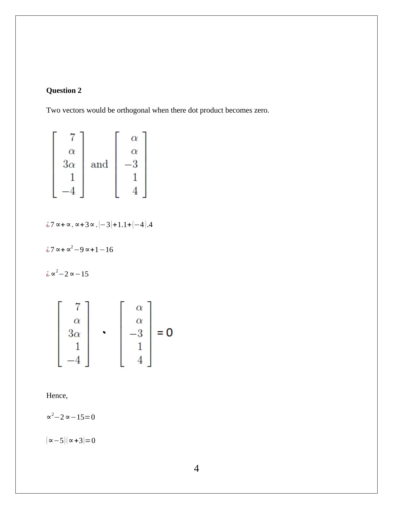
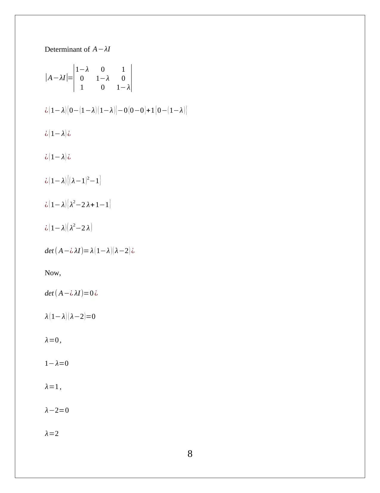
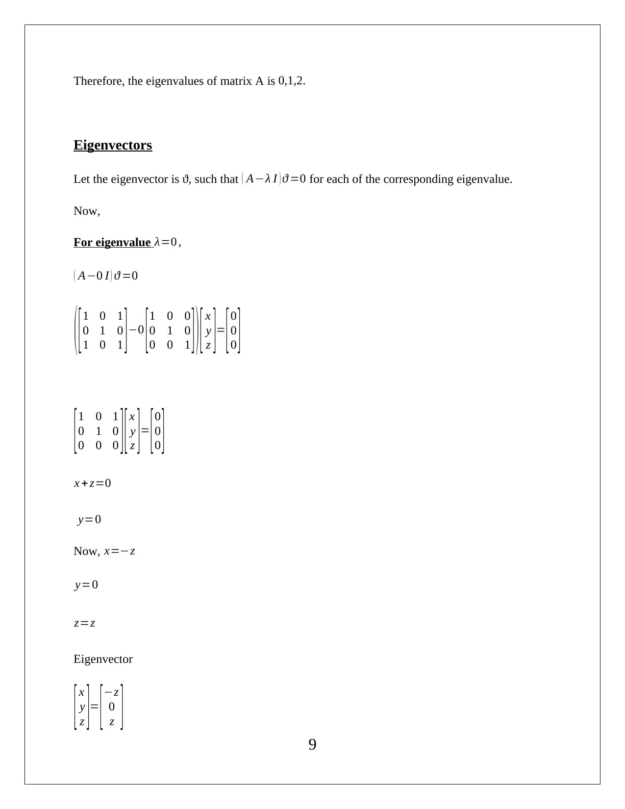
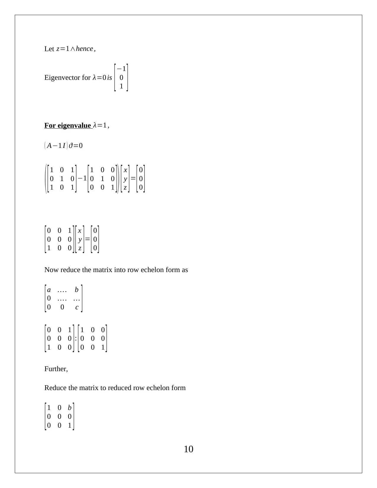
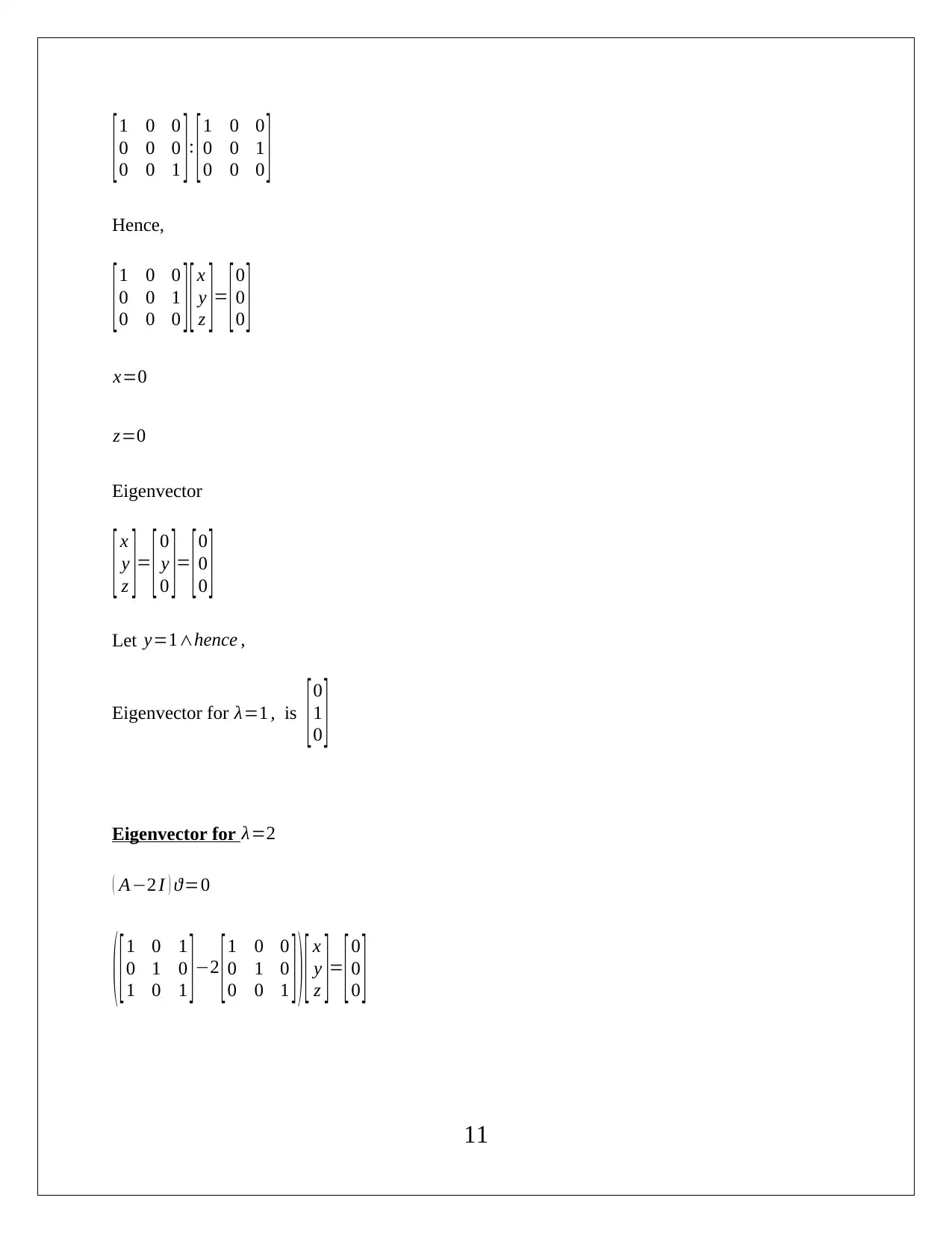
This document provides a detailed solution to SIT292 Linear Algebra Assignment 2 from 2017, covering key concepts such as matrix cofactors, orthogonal vectors, and the Gaussian elimination method. The solution includes step-by-step calculations and explanations for determining eigenvalues and eigenvectors for various matrices, along with verification steps. The assignment addresses concepts like matrix diagonalization and the conditions required for it. The solution also provides insights into matrix operations, systems of equations, and their consistency. This document is a valuable resource for students studying linear algebra, offering a comprehensive guide to solving complex problems and understanding the underlying principles.

SIT292 LINEAR ALGEBRA 2017
ASSIGNMENT 2
STUDENT ID
[Pick the date]

Question 1
(i) Given matrix
A=
[ 3 2 1
1 1 2
−1 −2 0 ]
 Cofactors Ci jof the matrix
Ci j=¿
C11=¿
C12 =¿
C13 =¿
C21 =¿
C22 =¿
C23 =¿
C31 =¿
C32 =¿
C33 =¿
Hence, cofactors of the matrix A would be given below:
1

Cofactors A= [ 4 −2 −1
−2 1 4
3 −5 1 ]
 Adj Aof the matrix A would be given below:
Adj A= [ 4 −2 3
−2 1 −5
−1 4 1 ]
(ii) Verification that computed adj Ais correct.
If A∗( adj A )
det A =I
Now,
LHS
A∗( adj A )= [ 3 2 1
1 1 2
−1 −2 0 ]. [ 4 −2 3
−2 1 −5
−1 4 1 ]
¿ [ 3.4+2. (−2)+1.(−1) 3.(−2)+2.1+1.4 3.3+ 2.(−5)+ 1.1
1.4+1.(−2)+2.(−1) 1.(−2)+1.1+2.4 1.3+ 1.(−5)+ 2.1
−1.4 +(−2) .(−2)+0.(−1) ( −1 ) . ( −2 ) +(−2).1+ 0.4 (−1).3+(−2). (−5)+ 0.1 ]
¿ [ 7 0 0
0 7 0
0 0 7 ]
And
A=
[ 3 2 1
1 1 2
−1 −2 0 ] 2

det A=
| 3 2 1
1 1 2
−1 −2 0|
¿ 3 ( 0+ 4 ) −2 ( 0+ 2 )+ 1 (−2+1 )
¿ 12−4−1
¿ 7
A∗( adj A )
det A =
[ 7 0 0
0 7 0
0 0 7 ]7 = [ 1 0 0
0 1 0
0 0 1 ]
RHS
I =
[1 0 0
0 1 0
0 0 1 ]
LHS = RHS
It is apparent that both the sides are equal and therefore, the computed adj A is correct.
3

Question 2
Two vectors would be orthogonal when there dot product becomes zero.
¿ 7 ∝+ ∝. ∝+3∝ . (−3 ) +1.1+ (−4 ) .4
¿ 7 ∝+ ∝2 −9 ∝+1−16
¿ ∝2−2 ∝−15
Hence,
∝2−2 ∝−15=0
( ∝−5 ) ( ∝+3 )=0
4

∝=5 ,−3
Therefore, the for ∝=5 ,−3the vectors would be orthogonal .
Question 3
Given equations
Gaussian elimination method to reduce the following system of equations into row echelon form
is applied below:
5

The row echelon form of the given system is given below:
This system does not have any solution because 0 ≠−5 .
It is apparent from the above that the given system has three linear equations and 4 variables.
Hence, the system is said to be inconsistent and does not have any solution as evident from the
above.
6

Question 4
Eigen values and eigenvectors of the given matrixes are as highlighted below:
 For matrix A
Eigen values
A=
[1 0 1
0 1 0
1 0 1 ]
Let λ is the eigenvalues of the given matrix in such a way that
det ( A−¿ λI )=0 ¿
Now,
A−λI = [1 0 1
0 1 0
1 0 1 ]−λ [1 0 0
0 1 0
0 0 1 ]
A−λI = [ 1 0 1
0 1 0
1 0 1 ] −
[|
λ 0 0
0 λ 0
0 0 λ|]
A−λI = [ 1−λ 0 1
0 1−λ 0
1 0 1−λ ]
7

Determinant of A−λI
|A−λI |=
|1−λ 0 1
0 1−λ 0
1 0 1− λ|
¿ ( 1− λ ) { 0− ( 1−λ ) ( 1−λ ) }−0 { 0−0 }+1 { 0− ( 1−λ ) }
¿ ( 1− λ ) ¿
¿ ( 1− λ ) ¿
¿ ( 1− λ ) { ( λ−1 )2−1 }
¿ ( 1− λ ) { λ2−2 λ+ 1−1 }
¿ ( 1− λ ) ( λ2−2 λ )
det ( A−¿ λI )= λ ( 1−λ ) ( λ−2 ) ¿
Now,
det ( A−¿ λI )=0 ¿
λ ( 1− λ ) ( λ−2 ) =0
λ=0 ,
1− λ=0
λ=1 ,
λ−2=0
λ=2
8

Therefore, the eigenvalues of matrix A is 0,1,2.
Eigenvectors
Let the eigenvector is ϑ, such that ( A−λ I ) ϑ =0 for each of the corresponding eigenvalue.
Now,
For eigenvalue λ=0 ,
( A−0 I ) ϑ =0
( [1 0 1
0 1 0
1 0 1 ]−0 [1 0 0
0 1 0
0 0 1 ] ) [ x
y
z ]= [0
0
0 ]
[1 0 1
0 1 0
0 0 0 ][ x
y
z ]= [0
0
0 ]
x + z=0
y=0
Now, x=−z
y=0
z=z
Eigenvector
[ x
y
z ]= [−z
0
z ] 9

Let z=1∧hence ,
Eigenvector for λ=0 is [−1
0
1 ]
For eigenvalue λ=1 ,
( A−1 I ) ϑ=0
( [1 0 1
0 1 0
1 0 1 ]−1 [1 0 0
0 1 0
0 0 1 ]) [ x
y
z ]= [0
0
0 ]
[0 0 1
0 0 0
1 0 0 ][ x
y
z ]= [0
0
0 ]
Now reduce the matrix into row echelon form as
[a … . b
0 … . …
0 0 c ]
[0 0 1
0 0 0
1 0 0 ]: [1 0 0
0 0 0
0 0 1 ]
Further,
Reduce the matrix to reduced row echelon form
[1 0 b
0 0 0
0 0 1 ] 10

[1 0 0
0 0 0
0 0 1 ]: [1 0 0
0 0 1
0 0 0 ]
Hence,
[1 0 0
0 0 1
0 0 0 ][ x
y
z ]= [0
0
0 ]
x=0
z=0
Eigenvector
[ x
y
z ]= [ 0
y
0 ]= [0
0
0 ]
Let y=1∧hence ,
Eigenvector for λ=1 , is [ 0
1
0 ]
Eigenvector for λ=2
( A−2 I ) ϑ=0
( [1 0 1
0 1 0
1 0 1 ]−2 [1 0 0
0 1 0
0 0 1 ] ) [ x
y
z ]= [0
0
0 ]
11

[−1 0 1
0 −1 0
1 0 −1 ][ x
y
z ]= [0
0
0 ]
Reduce the above matrix as
[a … b
0 .. …
0 0 c ]
[−1 0 1
0 −1 0
0 0 0 ]
Now reduce the matrix into reduced row echelon form as
[1 … b
0 .. …
0 0 1 ]
[1 0 −1
0 1 0
0 0 0 ]
[1 0 −1
0 1 0
0 0 0 ][ x
y
z ]= [0
0
0 ]
x−z=0
y=0
Now, x=z
y=0
12

z=z
Eigenvector
[ x
y
z ]= [ z
0
z ]
Let z=1∧hence ,
Eigenvector for λ=2 is [ 1
0
1 ]
Therefore, the eigenvectors of matrix A is [−1
0
1 ], [0
1
0 ], [1
0
1 ]
 For matrix B
Eigen values
B= [3 2 1
3 2 1
3 2 1 ]
Let λ is the eigenvalues of the given matrix in such a way that
det (B−¿ λI)=0 ¿
Now,
B−λI = [ 3 2 1
3 2 1
3 2 1 ]− λ [ 1 0 0
0 1 0
0 0 1 ]
13

B−λI = [ 3 2 1
3 2 1
3 2 1 ]−
[|
λ 0 0
0 λ 0
0 0 λ|]
B−λI = [ 3− λ 2 1
3 2−λ 1
3 2 1−λ ]
Determinant of B−λI
|B− λI|=
|3−λ 2 1
3 2−λ 1
3 2 1−λ |
¿ ( 3−λ ) ( λ2 −3 λ ) −2 (−3 λ ) +1.(3 λ)
¿− ( λ−6 ) λ2
det (B−¿ λI)=− ( λ−6 ) λ2 ¿
Now,
det (B−¿ λI)=0 ¿
− ( λ−6 ) λ2=0
( λ−6 ) λ2=0 ,
λ=0 ,
λ−6=0
λ=6
Therefore, the eigenvalues of matrix B is 0 , 6 .
14

Eigenvectors
Let the eigenvector is ϑ, such that ( B−λ I ) ϑ=0 for each of the corresponding eigenvalue.
Now,
For eigenvalue λ=0 ,
( B−0 I ) ϑ=0
( [3 2 1
3 2 1
3 2 1 ]−0 [1 0 0
0 1 0
0 0 1 ] ) [ x
y
z ]= [0
0
0 ]
[3 2 1
3 2 1
3 2 1 ][ x
y
z ]= [0
0
0 ]
Now reduce the matrix into row echelon form as
[a … . b
0 … . …
0 0 c ]
[3 2 1
3 2 1
3 2 1 ]: [3 2 1
0 0 0
0 0 0 ]
Now reduce the matrix into reduced row echelon form as
[1 0 b
0 0 0
0 0 1 ]
[ 3 2 1
0 0 0
0 0 0 ] :
[ 1 2
3
1
3
0 0 0
0 0 0 ] 15

Hence,
[ 1 2
3
1
3
0 0 0
0 0 0 ] [ x
y
z ]= [ 0
0
0 ]
x +( 2
3 ) y +( 1
3 ) z=0
x=− ( 2
3 ) y−( 1
3 ) z
Now,
Eigenvector
[ −( 2
3 ) y− ( 1
3 ) z
y
z ]=
[− ( 2
3 ) y
y
0 ] +
[− ( 1
3 ) z
0
z ] where , y∧z ≠ 0
Let y∧z =1
[−( 2
3 )
1
0 ] ,
[− ( 1
3 )
0
1 ]
Eigenvector for λ=0 is
[ −( 2
3 )
1
0 ] ,
[− ( 1
3 )
0
1 ]
For eigenvalue λ=6 ,
( B−0 I ) ϑ=0
16

( [3 2 1
3 2 1
3 2 1 ]−6 [1 0 0
0 1 0
0 0 1 ] ) [ x
y
z ]=
[0
0
0 ]
[ −3 2 1
3 −4 1
3 2 −5 ][ x
y
z ] = [ 0
0
0 ]
Now reduce the matrix into row echelon form as
[a … . b
0 … . …
0 0 c ]
[−3 2 1
3 −4 1
3 2 −5 ]: [−3 2 1
0 4 −4
0 0 0 ]
Now reduce the matrix into reduced row echelon form as
[1 0 b
0 0 0
0 0 1 ]
[ −3 2 1
0 4 −4
0 0 0 ] : [ 1 0 −1
0 1 −1
0 0 0 ]
Hence,
[1 0 −1
0 1 −1
0 0 0 ][ x
y
z ]= [0
0
0 ]
x−z=0
y−z =0
17

Now,
x=z
y=z
[ x
y
z ]= [ z
z
z ]
z ≠ 0∧hence let z=1
[ z
z
z ]= [1
1
1 ]
Eigenvector for λ=6 is [1
1
1 ]
Question 5
(a) Eigen values and eigenvectors of the given matrixes
Given
A=
[1 1 4
0 −1 1
0 0 2 ]
Let λ is the eigenvalues of the given matrix in such a way that
det ( A−¿ λI )=0 ¿
Now,
18

A−λI = [1 1 4
0 −1 1
0 0 2 ]−λ [1 0 0
0 1 0
0 0 1 ]
A−λI = [ 1 1 4
0 −1 1
0 0 2 ] − [ λ 0 0
0 λ 0
0 0 λ ]
A−λI = [1−λ 1 4
0 −1−λ 1
0 0 2−λ ]
Determinant of A−λI
| A−λI |=
|
1−λ 1 4
0 −1−λ 1
0 0 2−λ|
¿ ( 1− λ ) (λ2−λ−2)−1 {0−0 }+ 4 { 0−0 }
¿ ( 1− λ ) (λ−2)(λ+1)
det ( A−¿ λI )= ( 1−λ ) ( λ−2)( λ +1)¿
Now,
det ( A−¿ λI )=0 ¿
( 1− λ ) ( λ−2 ) ( λ+1 ) =0
1− λ=0 ,
λ=1 ,
λ−2=0
19

λ=2 ,
λ+1=0
λ=−1
Therefore, the eigenvalues of matrix A is 1 ,2 ,−1.
Eigenvectors
Let the eigenvector is ϑ, such that ( A−λ I ) ϑ =0 for each of the corresponding eigenvalue.
Now,
For eigenvalue λ=1 ,
( A−1 I ) ϑ=0
( [1 1 4
0 −1 1
0 0 2 ]−1 [1 0 0
0 1 0
0 0 1 ] ) [ x
y
z ]= [0
0
0 ]
[ 0 1 4
0 −2 1
0 0 1 ][ x
y
z ] =
[ 0
0
0 ]
Now reduce the matrix into row echelon form as
[1 … . b
0 … . …
0 0 1 ]
20

[ 0 1 4
0 −2 1
0 0 1 ] : [ 0 1 0
0 0 0
0 0 1 ]
Hence,
[0 1 0
0 0 0
0 0 1 ][ x
y
z ]= [0
0
0 ]
y=0
z=0
Now,
[ x
y
z ]= [ x
0
0 ]
Let x=1∧hence ,
Eigenvector for λ=0 is [1
0
0 ]
For eigenvalue λ=2 ,
( A−2 I ) ϑ=0
( [1 1 4
0 −1 1
0 0 2 ]−2 [1 0 0
0 1 0
0 0 1 ] ) [ x
y
z ]=
[0
0
0 ]
21

[−1 1 4
0 −3 1
0 0 0 ][ x
y
z ]=
[0
0
0 ]
Now reduce the matrix into row echelon form as
[1 … . b
0 … . …
0 0 1 ]
[−1 1 4
0 −3 1
0 0 0 ]: [−1 1 4
0 −3 1
0 0 0 ]
Now reduce the matrix into reduced row echelon form as
R 2← (−1
3 ) R 2
[ −1 1 4
0 1 −1
3
0 0 0 ]
R 1← R 1− ( 1. R 2 )
[ −1 0 13
3
0 1 −1
3
0 0 0 ]
R 1←−R1
[1 0 −13
3
0 1 −1
3
0 0 0 ] 22

Hence,
[1 0 −13
3
0 1 −1
3
0 0 0 ].
[ x
y
z ]= [0
0
0 ]
x− (13
3 )z =0
y− ( 1
3 ) z=0
And,
x= (13
3 )z ∧ y=( 1
3 )z
Now,
[ x
y
z ]=
[ ( 13
3 ) z
( 1
3 ) z
z ]
Let z=1∧hence ,
Eigenvector for λ=2 is
[ ( 13
3 )
( 1
3 )
1 ]
23

For eigenvalue λ=−1 ,
( A−(−1)I ) ϑ =0
( [1 1 4
0 −1 1
0 0 2 ]−(−1) [1 0 0
0 1 0
0 0 1 ] ) [ x
y
z ]=
[0
0
0 ]
[2 1 4
0 0 1
0 0 3 ][ x
y
z ]= [0
0
0 ]
Now reduce the matrix into row echelon form as
[1 … . b
0 … . …
0 0 1 ]
[ 2 1 4
0 0 1
0 0 3 ] :
[ 1 1
2 0
0 0 1
0 0 0 ]
Hence,
[1 1
2 0
0 0 1
0 0 0 ] [ x
y
z ]= [0
0
0 ]
x +( 1
2 ) y=0
z=0
Now,
24

x=− ( 1
2 ) y ∧z=0
[ x
y
z ]=
[−( 1
2 ) y
y
0 ]
Let y=1∧hence ,
Eigenvector for λ=−1 is
[ −( 1
2 )
1
0 ]
 For matrix B
B= [2 2 1
0 1 3
0 0 −1 ]
Let λ is the eigenvalues of the given matrix in such a way that
det (B−¿ λI)=0 ¿
Now,
B−λI = [2 2 1
0 1 3
0 0 −1 ]−λ [1 0 0
0 1 0
0 0 1 ]
B−λI = [2 2 1
0 1 3
0 0 −1 ]− [λ 0 0
0 λ 0
0 0 λ ] 25

B−λI = [2−λ 2 1
0 1− λ 3
0 0 −1−λ ]
Determinant of B−λI
|B− λI|=
|2−λ 2 1
0 1−λ 3
0 0 −1−λ |
¿ ( 2− λ ) (λ2−1)−2 { 0 } +1 { 0−0 }
¿ ( 2− λ ) (λ2−1)
det ( B−¿ λI )= ( 2−λ ) (λ2−1)¿
Now,
det (B−¿ λI)=0 ¿
( 2− λ ) (λ2−1)=0
( 2− λ ) ( λ−1 ) ( λ+1 ) =0 ,
λ=1 ,−1 , 2
Therefore, the eigenvalues of matrix A is 1 ,−1 , 2.
Eigenvectors
Let the eigenvector is ϑ, such that ( A−λ I ) ϑ =0 for each of the corresponding eigenvalue.
Now,
For eigenvalue λ=1 ,
26

( B−1 I ) ϑ =0
( [ 2 2 1
0 1 3
0 0 −1 ] −1 [ 1 0 0
0 1 0
0 0 1 ] ) [ x
y
z ] =
[ 0
0
0 ]
[ 1 2 1
0 0 3
0 0 −2 ][ x
y
z ] = [ 0
0
0 ]
Now reduce the matrix into row echelon form as
[1 … . b
0 … . …
0 0 1 ]
[ 1 2 1
0 0 3
0 0 −2 ] : [ 1 2 0
0 0 1
0 0 0 ]
Hence,
[1 2 0
0 0 1
0 0 0 ][ x
y
z ]= [0
0
0 ]
x +2 y =0 and x=−2 y
z=0
Now,
[ x
y
z ]= [−2 y
y
z ]
Let y=1∧hence ,
27

Eigenvector for λ=0 is [−2
1
0 ]
For eigenvalue λ=−1
( B−(−1) I ) ϑ=0
( [2 2 1
0 1 3
0 0 −1 ]−(−1) [1 0 0
0 1 0
0 0 1 ]) [ x
y
z ]= [0
0
0 ]
[3 2 1
0 2 3
0 0 0 ][ x
y
z ]= [0
0
0 ]
Now reduce the matrix into row echelon form as
[1 … . b
0 … . …
0 0 1 ]
[3 2 1
0 2 3
0 0 0 ]:
[1 0 −2
3
0 1 3
2
0 0 0 ]
Hence,
[ 1 0 −2
3
0 1 3
2
0 0 0 ] [ x
y
z ]= [ 0
0
0 ]
28

x− 2
3 z=0∧x= 2
3 z
y +( 3
2 )z=0∧ y =(−3
2 ) z
Now,
[ x
y
z ]=
[ 2
3 z
( −3
2 ) z
z ]
Let z=1∧hence ,
Eigenvector for λ=−1 is
[ 2
3
( 3
2 )
1 ]
For eigenvalue λ=2
( B−(2)I ) ϑ=0
( [ 2 2 1
0 1 3
0 0 −1 ] −(2) [ 1 0 0
0 1 0
0 0 1 ]) [ x
y
z ] = [ 0
0
0 ]
[ 0 2 1
0 −1 3
0 0 −3 ][ x
y
z ] = [ 0
0
0 ]
Now reduce the matrix into row echelon form as
29

[1 … . b
0 … . …
0 0 1 ]
[ 0 2 1
0 −1 3
0 0 −3 ] : [ 0 1 0
0 0 0
0 0 1 ]
Hence,
[0 1 0
0 0 0
0 0 1 ][ x
y
z ]= [0
0
0 ]
y=0
z=0
Now,
[ x
y
z ]= [ x
0
0 ]
Let x=1∧hence ,
Eigenvector for λ=2 is [ 1
0
0 ]
(b) Condition P−1 AP=B
Given matrix
A = [1 1 4
0 −1 1
0 0 2 ] 30

B= [2 2 1
0 1 3
0 0 −1 ]
In this case, the above condition would be fulfilled only when P would be and invertible matrix
and matrix B would be a diagonal matrix.
However, it is apparent from the above that matrix B is not a diagonal matrix and hence, matrix
P would not be determined for the condition P−1 AP=B .
Question 6
Given matrix
31

A = [3 2 −1
3 8 −3
3 6 −1 ]
(a) Eigenvalues of the given matrix
Let λ is the eigenvalues of the given matrix in such a way that
det ( A−¿ λI )=0 ¿
Now,
A−λI = [3 2 −1
3 8 −3
3 6 −1 ]− λ [1 0 0
0 1 0
0 0 1 ]
A−λI = [3 2 −1
3 8 −3
3 6 −1 ]− [ λ 0 0
0 λ 0
0 0 λ ]
A−λI = [3−λ 2 −1
3 8− λ −3
3 6 −1−λ ]
Determinant of A−λI
| A−λI |=
|
3−λ 2 −1
3 8−λ −3
3 6 −1−λ |
¿ ( 3−λ ) ( λ2 −7 λ+10 ) −2 ( 6−3 λ )−1 .3 ( λ−2 )
¿ ( 3−λ ) ( λ−2 ) ( λ−5 )−12+6 λ−3 λ+6
¿ ( 3−λ ) ( λ−2 ) ( λ−5 )+3 λ−6
¿ ( 3−λ ) ( λ−2 ) ( λ−5 )+3 ( λ−2 )
32

¿ ( λ−2 ) { ( 3− λ ) ( λ−5 ) + 3 }
¿ ( λ−2 ) { 3 λ−15−λ2+5 λ+ 3 }
¿ ( λ−2 ) {−λ2 +8 λ−12 }
¿− ( λ−2 ) { λ2−8 λ +12 }
¿− ( λ−2 ) ( λ−6 ) ( λ−2 )
det ( A−¿ λI )=− ( λ−2 ) ( λ−6 ) ( λ−2 ) ¿
Now,
det ( A−¿ λI )=0 ¿
− ( λ−2 ) ( λ−6 ) ( λ−2 ) =0
λ=2 ,2 , 6
Therefore, the eigenvalues of matrix A is 2 , 2, 6 .
(b) Eigenvectors for each of the eigenvalue
Eigenvectors
Let the eigenvector is ϑ, such that ( A−λ I ) ϑ =0 for each of the corresponding eigenvalue.
Now,
For eigenvalue λ=2 ,
( A−2 I ) ϑ=0
33

( [3 2 −1
3 8 −3
3 6 −1 ]−2 [1 0 0
0 1 0
0 0 1 ]) [ x
y
z ]= [0
0
0 ]
[1 2 −1
3 6 −3
3 6 −3 ][ x
y
z ]= [0
0
0 ]
Now reduce the matrix into row echelon form as
[a … . b
0 … . …
0 0 c ]
[ 1 2 −1
3 6 −3
3 6 −3 ] : [ 3 6 −3
0 0 0
0 0 0 ]
Now reduce the matrix into reduced row echelon form as
[1 … . b
0 … . …
0 0 1 ]
[3 6 −3
0 0 0
0 0 0 ]: [1 2 −1
0 0 0
0 0 0 ]
Hence,
[1 2 −1
0 0 0
0 0 0 ][ x
y
z ]= [0
0
0 ]
x +2 y −z=0 and x=−2 y + z
z=0
34

Now,
[ x
y
z ]= [−2 y +z
y
z ] or ¿ [
−2 y
y
0 ] + [ z
0
z ]
Where, y∧z ≠ 0
Let y=1∧z=1
hence ,
Eigenvector for λ=2 is [−2
1
0 ], [ 1
0
1 ]
For eigenvalue λ=6 ,
( A−2 I ) ϑ=0
( [3 2 −1
3 8 −3
3 6 −1 ]−6 [1 0 0
0 1 0
0 0 1 ] ) [ x
y
z ]= [0
0
0 ]
[−3 2 −1
3 2 −3
3 6 −7 ][ x
y
z ]= [0
0
0 ]
Now reduce the matrix into row echelon form as
[a … . b
0 … . …
0 0 c ]
[ −3 2 −1
3 2 −3
3 6 −7 ] : [ −3 2 −1
0 8 −8
0 0 0 ] 35

Now reduce the matrix into reduced row echelon form as
[1 … . b
0 … . …
0 0 1 ]
[ −3 2 −1
0 8 −8
0 0 0 ] :
[ 1 0 −1
3
0 1 −1
0 0 0 ]
Hence,
[ 1 0 −1
3
0 1 −1
0 0 0 ] [ x
y
z ]= [ 0
0
0 ]
x− ( 1
3 ) z =0 ,∨x= 1
3 z
y−z =0 ¿ y=z
Now,
[ x
y
z ]=
[ 1
3 z
z
z ]
Where, z ≠ 0
Let z=1
hence ,
36

Eigenvector for λ=6 is
[ 1
3
1
1 ]
Therefore, the eigenvectors are [ −2
1
0 ] , [ 1
0
1 ] ,
[ 1
3
1
1 ]
(c) Condition B=P−1 A P
Matrix P=?
Matrix A = [3 2 −1
3 8 −3
3 6 −1 ]
P matrix would be determined based on the eigenvectors of matrix A.
P=
[−2 1 1
3
1 0 1
0 1 1 ]
Now for Matrix B:
P−1=
[ −2 1 1
3
1 0 1
0 1 1 ]
−1
¿
[−2 1 1
3
1 0 1
0 1 1
⋮
1 0 0
0 1 0
0 0 1 ]
Now reduce matrix to row echelon form
37

[a … . b
0 … . …
0 0 c ]
R 2← R 2+( 1
2 ) R 1
[−2 1 1
3
0 1
2
7
6
0 1 1
⋮
1 0 0
1
2 1 0
0 0 1 ]
R 2↔ R 3
[ −2 1 1
3
0 1 1
0 1
2
7
6
⋮
1 0 0
0 0 1
1
2 1 0 ]
R 3 ← R 3− ( 1
2 )R 2
[ −2 1 1
3
0 1 1
0 0 2
3
⋮
1 0 0
0 0 1
1
2 1 −1
2 ]
Reduce the matrix to reduced row echelon form
[1 … . b
0 … . …
0 0 1 ]
38

[ 1 0 0
0 1 0
0 0 1
:
−3
4
−1
2
3
4
−3
4
−3
2
7
4
3
4
3
2
−3
4
]
P−1=
[−3
4
−1
2
3
4
−3
4
−3
2
7
4
3
4
3
2
−3
4
]
Now,
B=P−1 A P
¿
[ −3
4
−1
2
3
4
−3
4
−3
2
7
4
3
4
3
2
−3
4
] . [ 3 2 −1
3 8 −3
3 6 −1 ] .
[ −2 1 1
3
1 0 1
0 1 1 ]
¿
[−3
2 −1 3
2
−3
2 −3 7
2
9
2 9 −9
2 ].
[−2 1 1
3
1 0 1
0 1 1 ]
B= [ 2 0 0
0 2 0
0 0 6 ]
39

Hence, the matrix B is [2 0 0
0 2 0
0 0 6 ] .
To determine whether the computed matrix is correct on not based on the eigenvalues
determined in part (a).
If det (B) = multiplication of the eigenvalues
Now,
Debt ( B ) =
|
2 0 0
0 2 0
0 0 6|=2 ( 12 ) −0 ( 0 ) +0 ( 0 ) =24
Multiplication of the eigenvalues (From part a) = 2 * 2 * 6 = 24
It is apparent that both the sides are same and therefore, the computed matrix B is correct.
40

41