Linear Algebra A32-A34: Matrices, Transformations, and Null Spaces

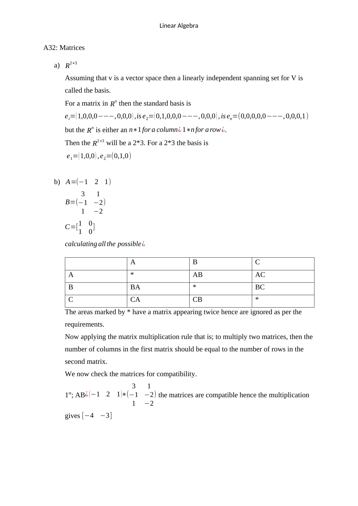
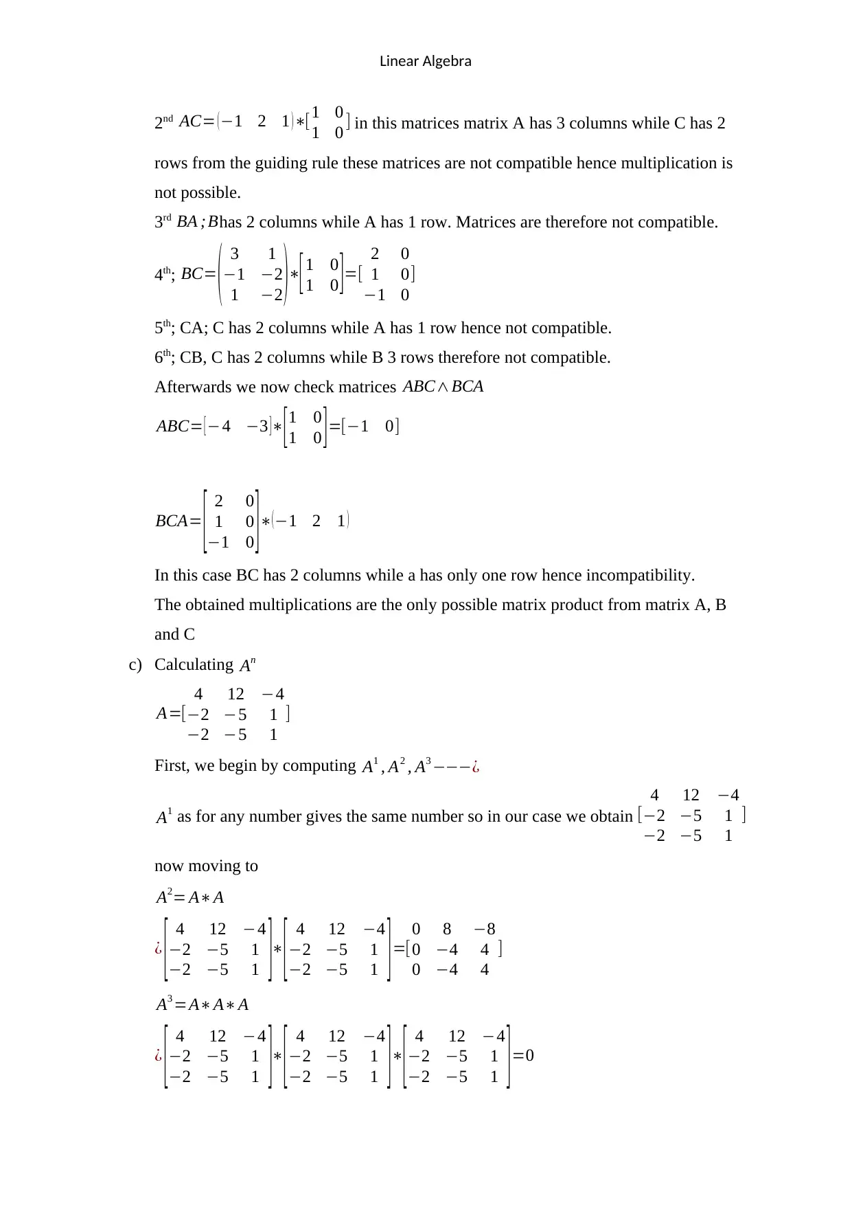
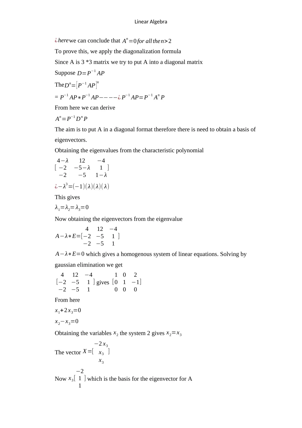
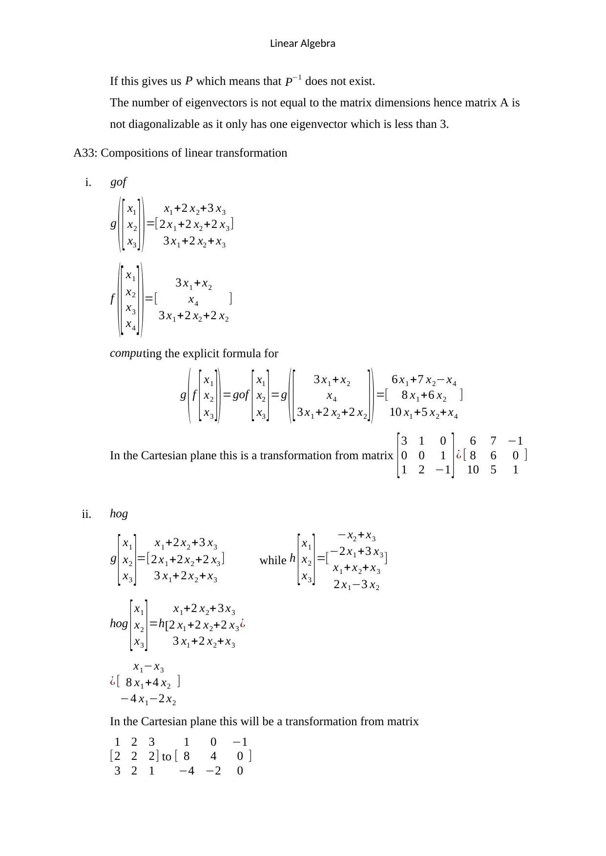
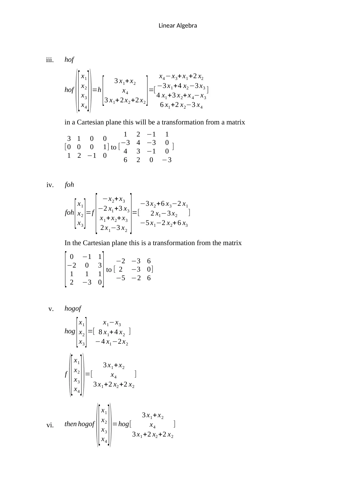
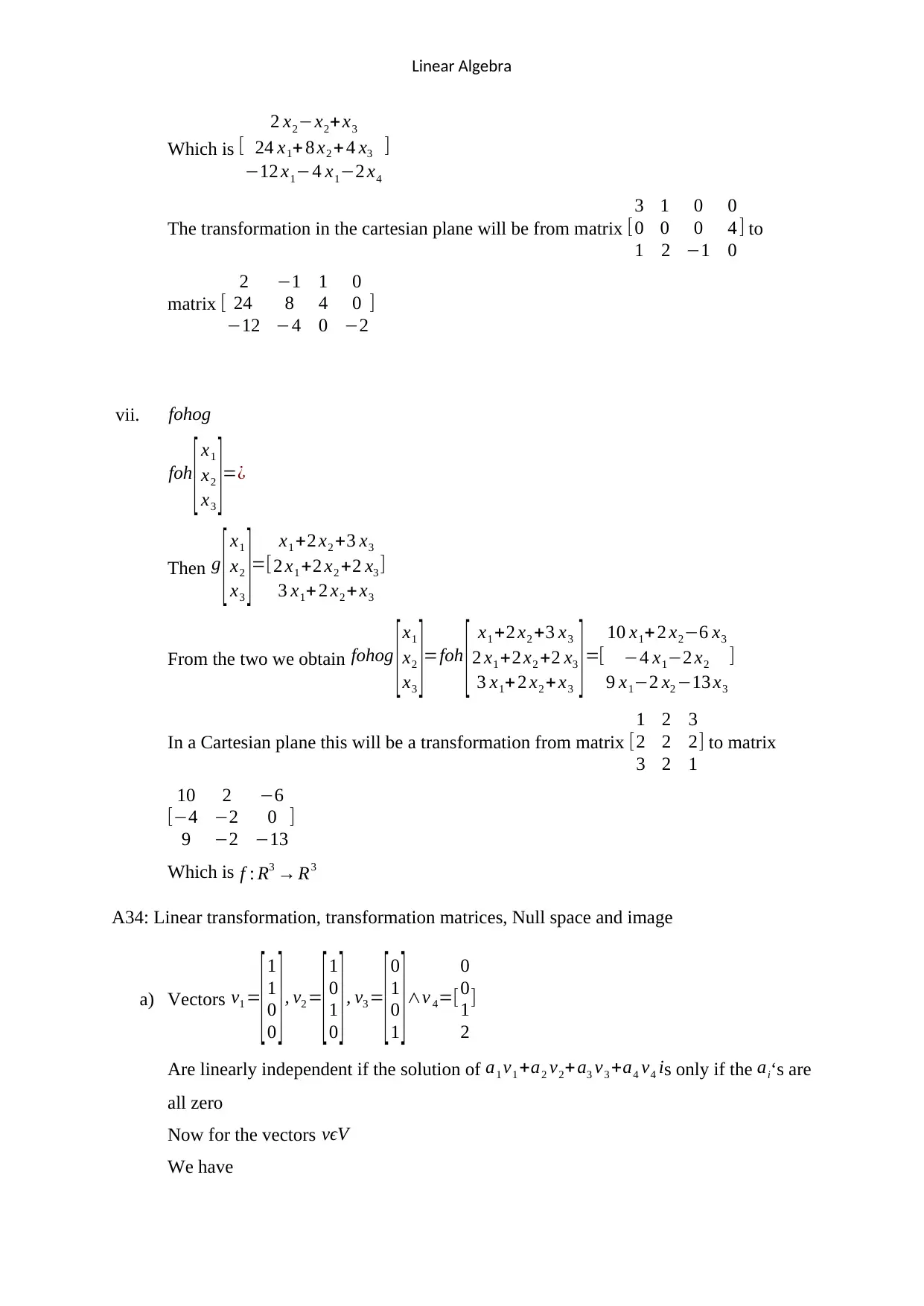
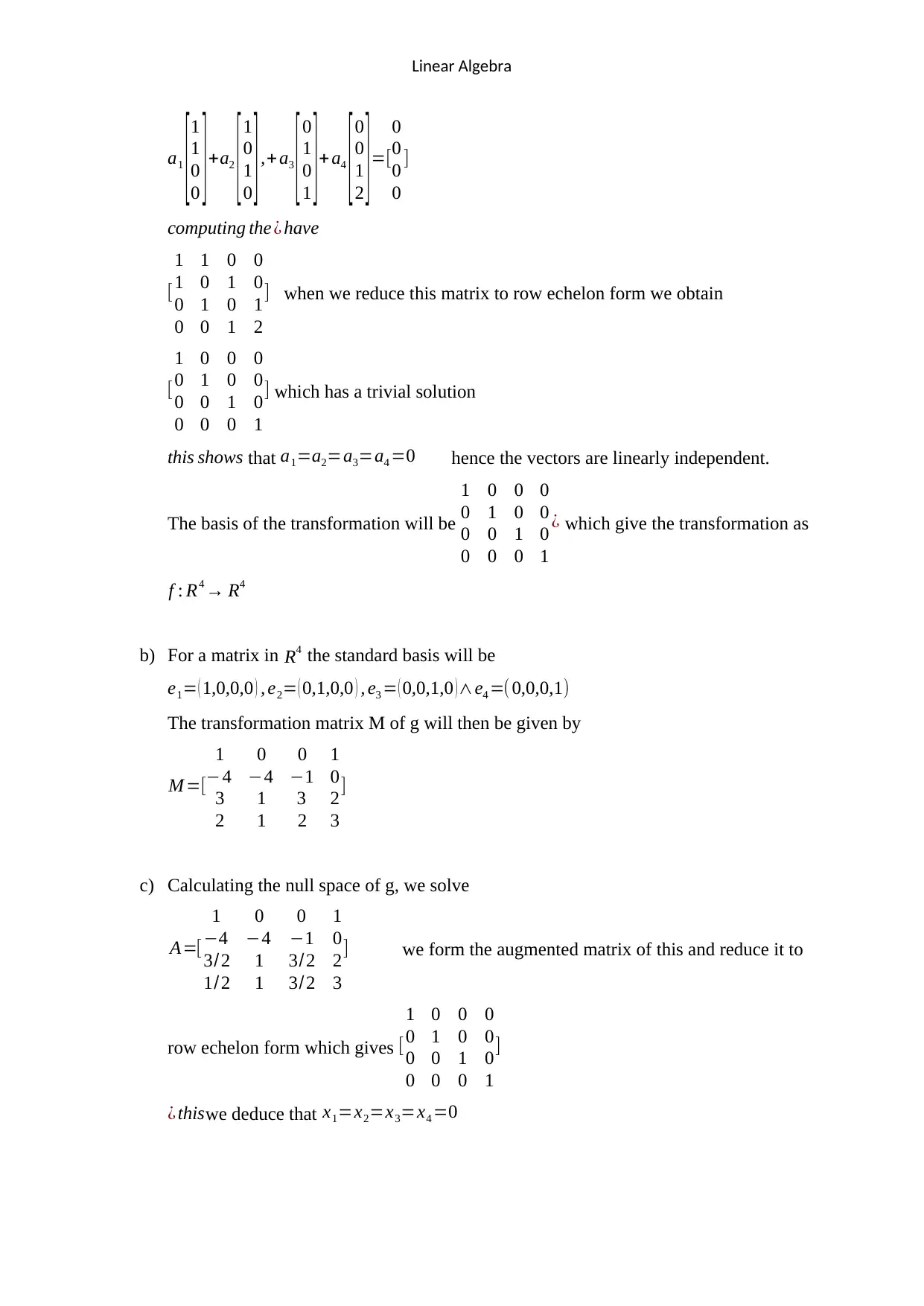
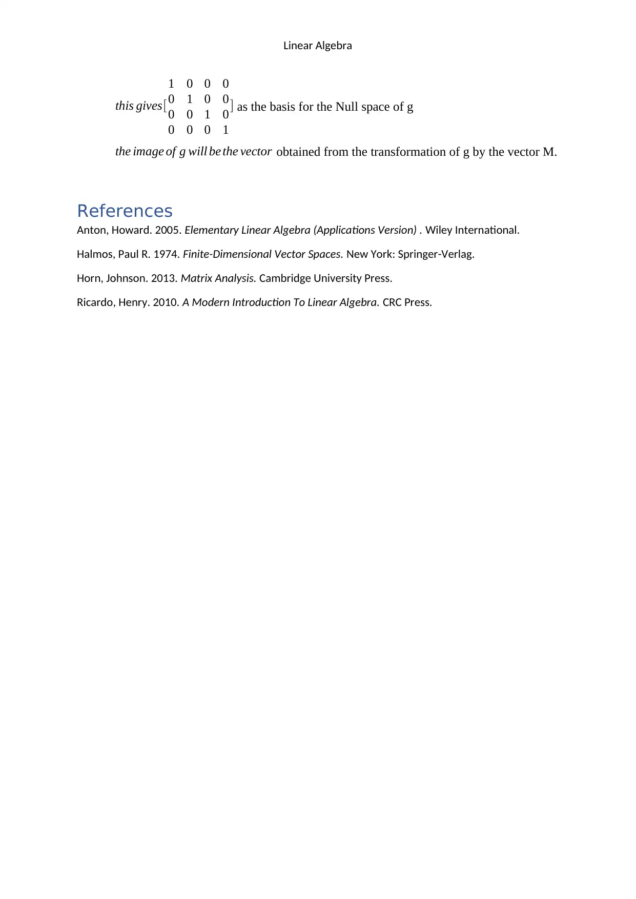
This document provides solutions to a Linear Algebra assignment (A32-A34) covering key concepts such as matrices, vector spaces, and linear transformations. The solution begins by analyzing matrix multiplication rules and compatibility, specifically addressing the standard basis of a matrix and the basis for a 2x3 matrix, including the multiplication of matrices and checking for compatibility. It then proceeds to prove the diagonalization of a matrix, including the computation of eigenvalues and eigenvectors, and demonstrating when a matrix is not diagonalizable. Further, it covers compositions of linear transformations and their matrix representations in the Cartesian plane, including calculations for various transformations. The solution concludes with an analysis of linear independence, determining the transformation matrix, and calculating the null space of a given transformation. The assignment is supported by several references to established linear algebra textbooks.

Linear Algebra
A32: Matrices
a) R2∗3
Assuming that v is a vector space then a linearly independent spanning set for V is
called the basis.
For a matrix in Rn then the standard basis is
ei= ( 1,0,0,0−−−, 0,0,0 ) ,is e2= ( 0,1,0,0,0−−−, 0,0,0 ) , is en=(0,0,0,0,0−−−, 0,0,0,1)
but the Rn is either an n∗1 for a column¿ 1∗n for a row ¿.
Then the R2∗3 will be a 2*3. For a 2*3 the basis is
e1= ( 1,0,0 ) , e2=(0,1,0)
b) A=(−1 2 1)
B=(
3 1
−1 −2
1 −2
)
C=[1 0
1 0]
calculating all the possible¿
A B C
A * AB AC
B BA * BC
C CA CB *
The areas marked by * have a matrix appearing twice hence are ignored as per the
requirements.
Now applying the matrix multiplication rule that is; to multiply two matrices, then the
number of columns in the first matrix should be equal to the number of rows in the
second matrix.
We now check the matrices for compatibility.
1st; AB¿ ( −1 2 1 )∗(
3 1
−1 −2
1 −2
) the matrices are compatible hence the multiplication
gives [−4 −3]

Linear Algebra
2nd AC= (−1 2 1 )∗[1 0
1 0 ] in this matrices matrix A has 3 columns while C has 2
rows from the guiding rule these matrices are not compatible hence multiplication is
not possible.
3rd BA ; Bhas 2 columns while A has 1 row. Matrices are therefore not compatible.
4th; BC= ( 3 1
−1 −2
1 −2 )∗[1 0
1 0 ]=[
2 0
1 0
−1 0
]
5th; CA; C has 2 columns while A has 1 row hence not compatible.
6th; CB, C has 2 columns while B 3 rows therefore not compatible.
Afterwards we now check matrices ABC∧BCA
ABC= [ −4 −3 ]∗
[ 1 0
1 0 ] =[−1 0]
BCA= [ 2 0
1 0
−1 0 ]∗( −1 2 1 )
In this case BC has 2 columns while a has only one row hence incompatibility.
The obtained multiplications are the only possible matrix product from matrix A, B
and C
c) Calculating An
A=[
4 12 −4
−2 −5 1
−2 −5 1
]
First, we begin by computing A1 , A2 , A3 −−−¿
A1 as for any number gives the same number so in our case we obtain [
4 12 −4
−2 −5 1
−2 −5 1
]
now moving to
A2= A∗A
¿ [ 4 12 −4
−2 −5 1
−2 −5 1 ]∗
[ 4 12 −4
−2 −5 1
−2 −5 1 ]=[
0 8 −8
0 −4 4
0 −4 4
]
A3 =A∗A∗A
¿ [ 4 12 −4
−2 −5 1
−2 −5 1 ]∗
[ 4 12 −4
−2 −5 1
−2 −5 1 ]∗
[ 4 12 −4
−2 −5 1
−2 −5 1 ]=0

Linear Algebra
¿ herewe can conclude that An =0 for all then>2
To prove this, we apply the diagonalization formula
Since A is 3 *3 matrix we try to put A into a diagonal matrix
Suppose D=P−1 AP
TheDn= [ P−1 AP ]n
= P−1 AP∗P−1 AP−−−−¿ P−1 AP=P−1 An P
From here we can derive
An =P−1 Dn P
The aim is to put A in a diagonal format therefore there is need to obtain a basis of
eigenvectors.
Obtaining the eigenvalues from the characteristic polynomial
[
4−λ 12 −4
−2 −5−λ 1
−2 −5 1−λ
]
¿−λ3 =(−1)( λ)( λ)( λ)
This gives
λ1=λ2= λ3=0
Now obtaining the eigenvectors from the eigenvalue
A−λ∗E=[
4 12 −4
−2 −5 1
−2 −5 1
]
A−λ∗E=0 which gives a homogenous system of linear equations. Solving by
gaussian elimination we get
[
4 12 −4
−2 −5 1
−2 −5 1
] gives [
1 0 2
0 1 −1
0 0 0
]
From here
x1+ 2 x3=0
x2−x3=0
Obtaining the variables x2 the system 2 gives x2=x3
The vector X =[
−2 x3
x3
x3
]
Now x3 [
−2
1
1
] which is the basis for the eigenvector for A

Linear Algebra
If this gives us P which means that P−1 does not exist.
The number of eigenvectors is not equal to the matrix dimensions hence matrix A is
not diagonalizable as it only has one eigenvector which is less than 3.
A33: Compositions of linear transformation
i. gοf
g
( [ x1
x2
x3
] )=[
x1 +2 x2+3 x3
2 x1 +2 x2 +2 x3
3 x1 +2 x2 + x3
]
f
([ x1
x2
x3
x4
] )=[
3 x1 +x2
x4
3 x1 +2 x2 +2 x2
]
computing the explicit formula for
g
(f
[ x1
x2
x3
])=gοf
[ x1
x2
x3
]=g
( [ 3 x1 + x2
x4
3 x1 +2 x2 +2 x2
] )=[
6 x1 +7 x2−x4
8 x1 +6 x2
10 x1 +5 x2+x4
]
In the Cartesian plane this is a transformation from matrix [3 1 0
0 0 1
1 2 −1 ]¿ [
6 7 −1
8 6 0
10 5 1
]
ii. hοg
g
[ x1
x2
x3 ]=[
x1 +2 x2 +3 x3
2 x1 +2 x2 +2 x3
3 x1+ 2 x2 + x3
] while h
[x1
x2
x3
]=[
−x2 +x3
−2 x1 +3 x3
x1 +x2+x3
2 x1−3 x2
]
hοg
[x1
x2
x3 ]=h[
x1+2 x2+3 x3
2 x1 +2 x2+2 x3
3 x1 +2 x2+ x3
¿
¿ [
x1−x3
8 x1 +4 x2
−4 x1−2 x2
]
In the Cartesian plane this will be a transformation from matrix
[
1 2 3
2 2 2
3 2 1
] to [
1 0 −1
8 4 0
−4 −2 0
]

Linear Algebra
iii. hοf
hοf
( [ x1
x2
x3
x4
] )=h
[ 3 x1+x2
x4
3 x1+2 x2 +2 x2 ]=[
x4 −x3+ x1 +2 x2
−3 x1 +4 x2 −3 x3
4 x1 +3 x2+x 4−x3
6 x1 +2 x2−3 x4
]
in a Cartesian plane this will be a transformation from a matrix
[
3 1 0 0
0 0 0 1
1 2 −1 0
] to [
1 2 −1 1
−3 4 −3 0
4 3 −1 0
6 2 0 −3
]
iv. fοh
fοh
[ x1
x2
x3 ]=f
[ −x2+x3
−2 x1 +3 x3
x1 + x2+ x3
2 x1−3 x2
]=[
−3 x2 +6 x3−2 x1
2 x1−3 x2
−5 x1−2 x2+ 6 x3
]
In the Cartesian plane this is a transformation from the matrix
[ 0 −1 1
−2 0 3
1 1 1
2 −3 0 ] to [
−2 −3 6
2 −3 0
−5 −2 6
]
v. hοgοf
hοg
[x1
x2
x3 ]=[
x1−x3
8 x1+ 4 x2
−4 x1 −2 x2
]
f
([ x1
x2
x3
x4
] )=[
3 x1 +x2
x4
3 x1 +2 x2 +2 x2
]
vi. then hοgοf
([ x1
x2
x3
x4
] )=hοg[
3 x1 + x2
x4
3 x1 +2 x2 +2 x2
]

Linear Algebra
Which is [
2 x2−x2+x3
24 x1+ 8 x2 + 4 x3
−12 x1−4 x1−2 x4
]
The transformation in the cartesian plane will be from matrix [
3 1 0 0
0 0 0 4
1 2 −1 0
] to
matrix [
2 −1 1 0
24 8 4 0
−12 −4 0 −2
]
vii. fοhοg
fοh
[ x1
x2
x3 ]=¿
Then g
[ x1
x2
x3 ]=[
x1 +2 x2 +3 x3
2 x1 +2 x2 +2 x3
3 x1+ 2 x2 + x3
]
From the two we obtain fοhοg
[x1
x2
x3 ]=fοh
[ x1 +2 x2 +3 x3
2 x1 +2 x2 +2 x3
3 x1+ 2 x2 +x3 ]=[
10 x1+ 2 x2−6 x3
−4 x1−2 x2
9 x1−2 x2 −13 x3
]
In a Cartesian plane this will be a transformation from matrix [
1 2 3
2 2 2
3 2 1
] to matrix
[
10 2 −6
−4 −2 0
9 −2 −13
]
Which is f : R3 → R3
A34: Linear transformation, transformation matrices, Null space and image
a) Vectors v1 =
[1
1
0
0 ], v2 =
[1
0
1
0 ], v3 =
[0
1
0
1 ]∧v 4=[
0
0
1
2
]
Are linearly independent if the solution of a1 v1 +a2 v2+ a3 v3 +a4 v4 is only if the ai‘s are
all zero
Now for the vectors vϵV
We have

Linear Algebra
a1
[1
1
0
0 ]+a2
[1
0
1
0 ],+a3
[0
1
0
1 ]+ a4
[0
0
1
2 ]=[
0
0
0
0
]
computing the¿ have
[
1 1 0 0
1 0 1 0
0 1 0 1
0 0 1 2
] when we reduce this matrix to row echelon form we obtain
[
1 0 0 0
0 1 0 0
0 0 1 0
0 0 0 1
] which has a trivial solution
this shows that a1=a2=a3=a4 =0 hence the vectors are linearly independent.
The basis of the transformation will be
1 0 0 0
0 1 0 0
0 0 1 0
0 0 0 1
¿ which give the transformation as
f : R4 → R4
b) For a matrix in R4 the standard basis will be
e1= ( 1,0,0,0 ) , e2= ( 0,1,0,0 ) , e3 = ( 0,0,1,0 )∧e4 =( 0,0,0,1)
The transformation matrix M of g will then be given by
M =[
1 0 0 1
−4 −4 −1 0
3 1 3 2
2 1 2 3
]
c) Calculating the null space of g, we solve
A=[
1 0 0 1
−4 −4 −1 0
3/2 1 3/2 2
1/2 1 3/2 3
] we form the augmented matrix of this and reduce it to
row echelon form which gives [
1 0 0 0
0 1 0 0
0 0 1 0
0 0 0 1
]
¿ thiswe deduce that x1=x2=x3=x4 =0

Linear Algebra
this gives[
1 0 0 0
0 1 0 0
0 0 1 0
0 0 0 1
] as the basis for the Null space of g
the image of g will be the vector obtained from the transformation of g by the vector M.
References
Anton, Howard. 2005. Elementary Linear Algebra (Applications Version) . Wiley International.
Halmos, Paul R. 1974. Finite-Dimensional Vector Spaces. New York: Springer-Verlag.
Horn, Johnson. 2013. Matrix Analysis. Cambridge University Press.
Ricardo, Henry. 2010. A Modern Introduction To Linear Algebra. CRC Press.