Linear Programming Model in Excel Solver: Production Planning

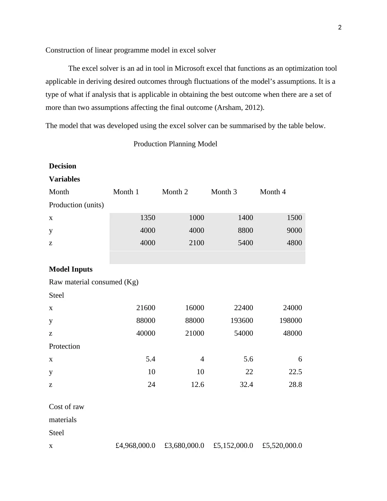
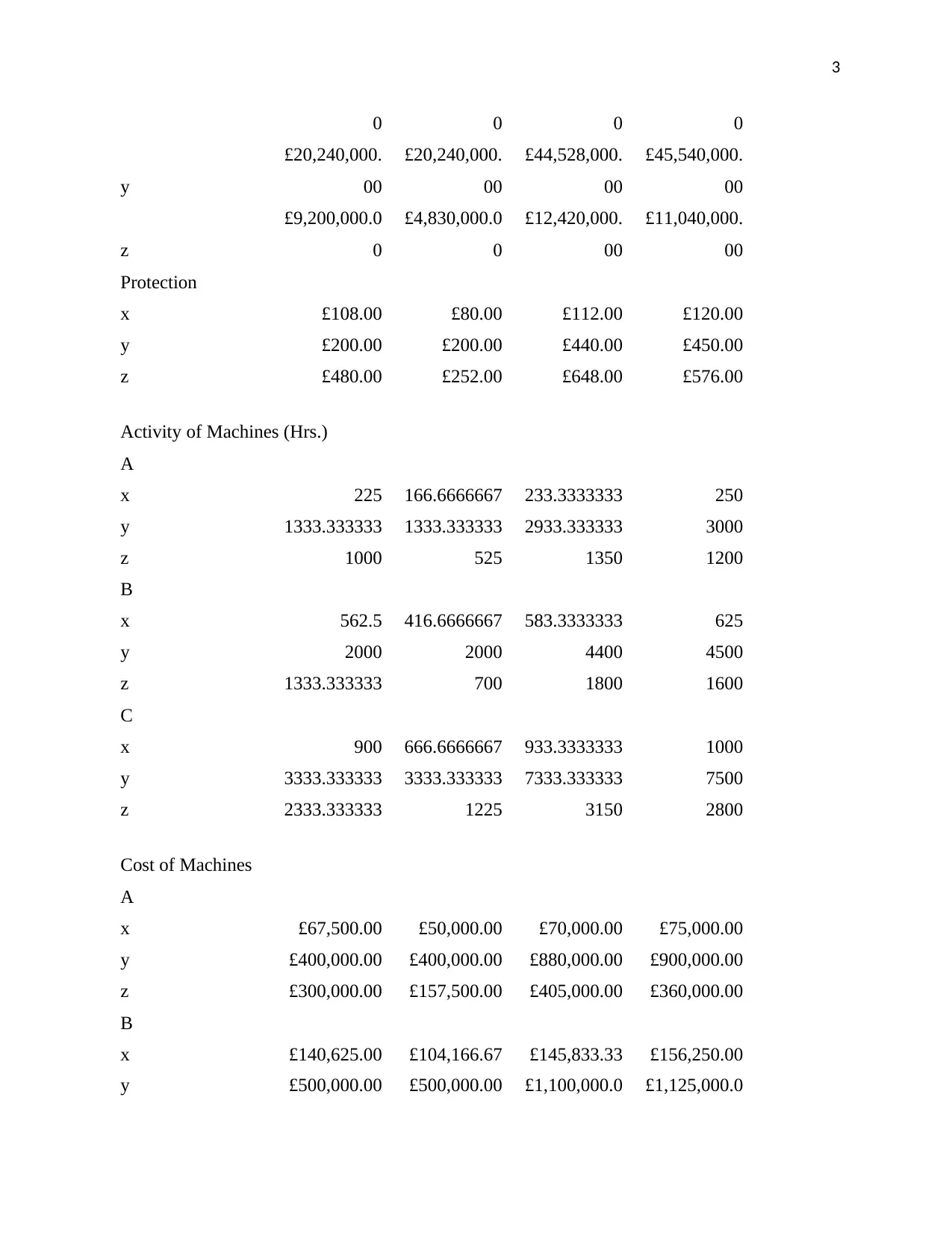
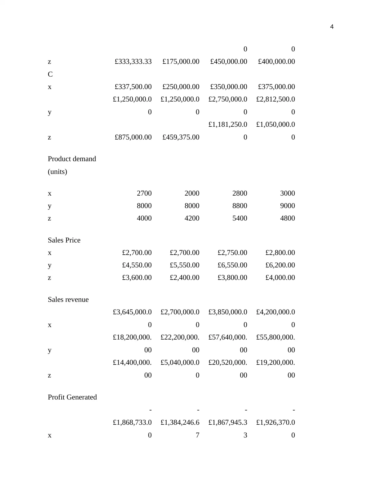
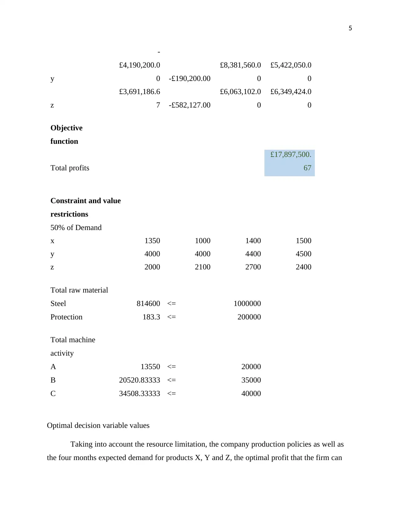
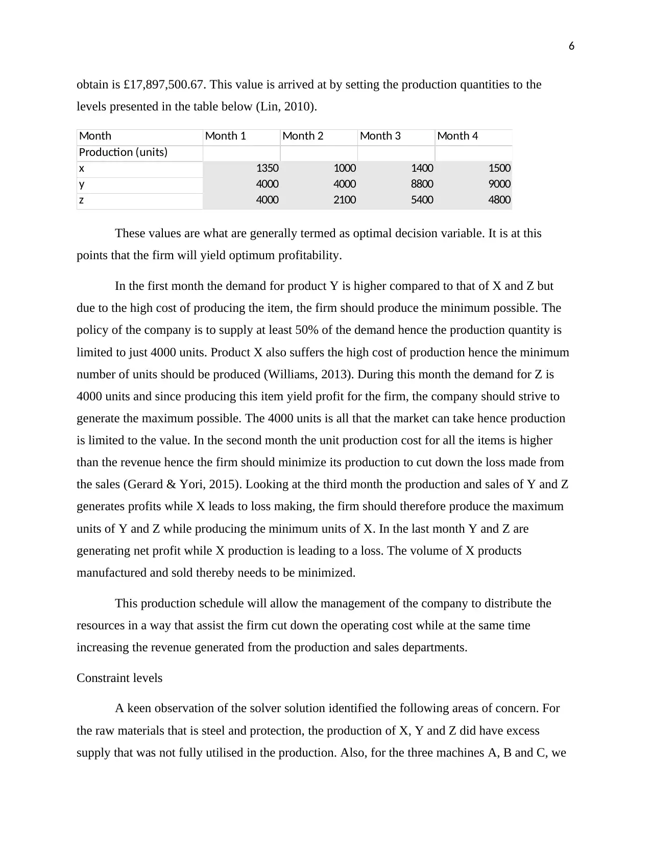
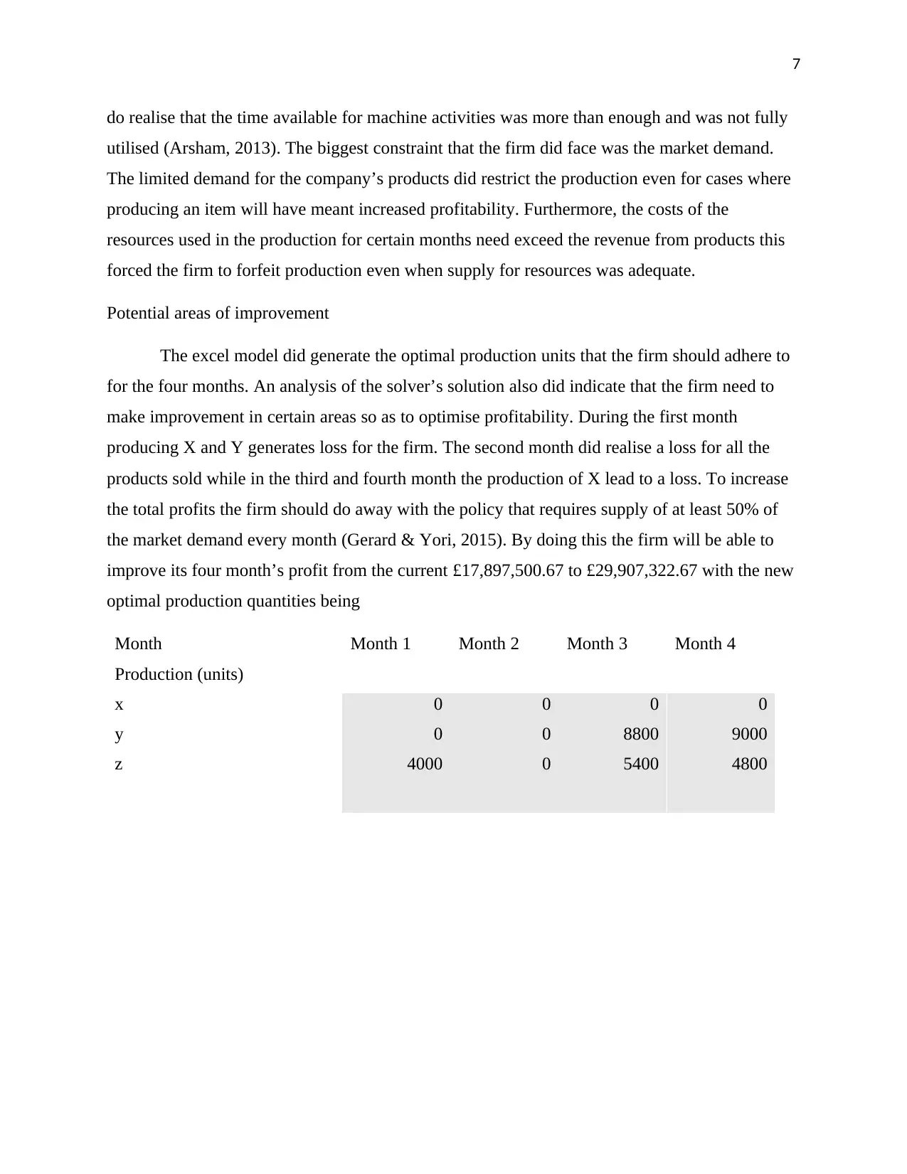
This assignment presents a linear programming model constructed using Excel Solver to optimize production planning for a company producing three products (X, Y, and Z) over four months. The model incorporates decision variables, model inputs such as raw material consumption, production costs, machine activity, and product demand to determine the optimal production quantities for each product each month. The objective is to maximize total profits, subject to constraints including resource limitations and market demand. The solution details the optimal decision variable values, analyzes constraint levels, and identifies potential areas for improvement, such as eliminating the policy of supplying at least 50% of market demand to increase overall profitability. The analysis highlights how the company can adjust production schedules to reduce operating costs and boost revenue, ultimately achieving an optimal profit of £17,897,500.67, or potentially £29,907,322.67 with revised production quantities.

1
Linear Algebra
Student Name
Institution Name

2
Construction of linear programme model in excel solver
The excel solver is an ad in tool in Microsoft excel that functions as an optimization tool
applicable in deriving desired outcomes through fluctuations of the model’s assumptions. It is a
type of what if analysis that is applicable in obtaining the best outcome when there are a set of
more than two assumptions affecting the final outcome (Arsham, 2012).
The model that was developed using the excel solver can be summarised by the table below.
Production Planning Model
Decision
Variables
Month Month 1 Month 2 Month 3 Month 4
Production (units)
x 1350 1000 1400 1500
y 4000 4000 8800 9000
z 4000 2100 5400 4800
Model Inputs
Raw material consumed (Kg)
Steel
x 21600 16000 22400 24000
y 88000 88000 193600 198000
z 40000 21000 54000 48000
Protection
x 5.4 4 5.6 6
y 10 10 22 22.5
z 24 12.6 32.4 28.8
Cost of raw
materials
Steel
x £4,968,000.0 £3,680,000.0 £5,152,000.0 £5,520,000.0

3
0 0 0 0
y
£20,240,000.
00
£20,240,000.
00
£44,528,000.
00
£45,540,000.
00
z
£9,200,000.0
0
£4,830,000.0
0
£12,420,000.
00
£11,040,000.
00
Protection
x £108.00 £80.00 £112.00 £120.00
y £200.00 £200.00 £440.00 £450.00
z £480.00 £252.00 £648.00 £576.00
Activity of Machines (Hrs.)
A
x 225 166.6666667 233.3333333 250
y 1333.333333 1333.333333 2933.333333 3000
z 1000 525 1350 1200
B
x 562.5 416.6666667 583.3333333 625
y 2000 2000 4400 4500
z 1333.333333 700 1800 1600
C
x 900 666.6666667 933.3333333 1000
y 3333.333333 3333.333333 7333.333333 7500
z 2333.333333 1225 3150 2800
Cost of Machines
A
x £67,500.00 £50,000.00 £70,000.00 £75,000.00
y £400,000.00 £400,000.00 £880,000.00 £900,000.00
z £300,000.00 £157,500.00 £405,000.00 £360,000.00
B
x £140,625.00 £104,166.67 £145,833.33 £156,250.00
y £500,000.00 £500,000.00 £1,100,000.0 £1,125,000.0

4
0 0
z £333,333.33 £175,000.00 £450,000.00 £400,000.00
C
x £337,500.00 £250,000.00 £350,000.00 £375,000.00
y
£1,250,000.0
0
£1,250,000.0
0
£2,750,000.0
0
£2,812,500.0
0
z £875,000.00 £459,375.00
£1,181,250.0
0
£1,050,000.0
0
Product demand
(units)
x 2700 2000 2800 3000
y 8000 8000 8800 9000
z 4000 4200 5400 4800
Sales Price
x £2,700.00 £2,700.00 £2,750.00 £2,800.00
y £4,550.00 £5,550.00 £6,550.00 £6,200.00
z £3,600.00 £2,400.00 £3,800.00 £4,000.00
Sales revenue
x
£3,645,000.0
0
£2,700,000.0
0
£3,850,000.0
0
£4,200,000.0
0
y
£18,200,000.
00
£22,200,000.
00
£57,640,000.
00
£55,800,000.
00
z
£14,400,000.
00
£5,040,000.0
0
£20,520,000.
00
£19,200,000.
00
Profit Generated
x
-
£1,868,733.0
0
-
£1,384,246.6
7
-
£1,867,945.3
3
-
£1,926,370.0
0

5
y
-
£4,190,200.0
0 -£190,200.00
£8,381,560.0
0
£5,422,050.0
0
z
£3,691,186.6
7 -£582,127.00
£6,063,102.0
0
£6,349,424.0
0
Objective
function
Total profits
£17,897,500.
67
Constraint and value
restrictions
50% of Demand
x 1350 1000 1400 1500
y 4000 4000 4400 4500
z 2000 2100 2700 2400
Total raw material
Steel 814600 <= 1000000
Protection 183.3 <= 200000
Total machine
activity
A 13550 <= 20000
B 20520.83333 <= 35000
C 34508.33333 <= 40000
Optimal decision variable values
Taking into account the resource limitation, the company production policies as well as
the four months expected demand for products X, Y and Z, the optimal profit that the firm can

6
obtain is £17,897,500.67. This value is arrived at by setting the production quantities to the
levels presented in the table below (Lin, 2010).
Month Month 1 Month 2 Month 3 Month 4
Production (units)
x 1350 1000 1400 1500
y 4000 4000 8800 9000
z 4000 2100 5400 4800
These values are what are generally termed as optimal decision variable. It is at this
points that the firm will yield optimum profitability.
In the first month the demand for product Y is higher compared to that of X and Z but
due to the high cost of producing the item, the firm should produce the minimum possible. The
policy of the company is to supply at least 50% of the demand hence the production quantity is
limited to just 4000 units. Product X also suffers the high cost of production hence the minimum
number of units should be produced (Williams, 2013). During this month the demand for Z is
4000 units and since producing this item yield profit for the firm, the company should strive to
generate the maximum possible. The 4000 units is all that the market can take hence production
is limited to the value. In the second month the unit production cost for all the items is higher
than the revenue hence the firm should minimize its production to cut down the loss made from
the sales (Gerard & Yori, 2015). Looking at the third month the production and sales of Y and Z
generates profits while X leads to loss making, the firm should therefore produce the maximum
units of Y and Z while producing the minimum units of X. In the last month Y and Z are
generating net profit while X production is leading to a loss. The volume of X products
manufactured and sold thereby needs to be minimized.
This production schedule will allow the management of the company to distribute the
resources in a way that assist the firm cut down the operating cost while at the same time
increasing the revenue generated from the production and sales departments.
Constraint levels
A keen observation of the solver solution identified the following areas of concern. For
the raw materials that is steel and protection, the production of X, Y and Z did have excess
supply that was not fully utilised in the production. Also, for the three machines A, B and C, we

7
do realise that the time available for machine activities was more than enough and was not fully
utilised (Arsham, 2013). The biggest constraint that the firm did face was the market demand.
The limited demand for the company’s products did restrict the production even for cases where
producing an item will have meant increased profitability. Furthermore, the costs of the
resources used in the production for certain months need exceed the revenue from products this
forced the firm to forfeit production even when supply for resources was adequate.
Potential areas of improvement
The excel model did generate the optimal production units that the firm should adhere to
for the four months. An analysis of the solver’s solution also did indicate that the firm need to
make improvement in certain areas so as to optimise profitability. During the first month
producing X and Y generates loss for the firm. The second month did realise a loss for all the
products sold while in the third and fourth month the production of X lead to a loss. To increase
the total profits the firm should do away with the policy that requires supply of at least 50% of
the market demand every month (Gerard & Yori, 2015). By doing this the firm will be able to
improve its four month’s profit from the current £17,897,500.67 to £29,907,322.67 with the new
optimal production quantities being
Month Month 1 Month 2 Month 3 Month 4
Production (units)
x 0 0 0 0
y 0 0 8800 9000
z 4000 0 5400 4800

8
References
Arsham, H., 2012. Foundation of linear programming: A managerial perspective from solvingsystem of
inequalities to software implementation. International Journal of Strategic Decision Sciences,
3(3), p. 40–60.
Arsham, H., 2013. An interior boundary pivotal solution algorithm for linear programs with the optimal
solution-based sensitivity region. International Journal of Mathematics in Operational
Research.
Gerard, S. & Diptesh, G., 2010. Networks in Action; Text and Computer Exercises in Network
Optimization, s.l.: Springer.
Gerard, S. & Yori, Z., 2015. Linear and Integer Optimization: Theory and Practice, s.l.: CRC Press.
Lin, C., 2010. Computing shadow proces/costs of dengernerate LP problems with reduced simplex
tables. Expert Systems with Applicationsplex tables, Volume 37, p. 5848–5855..
Wang, J., 2014. Management Science, Logistics, and Operations Research. 2014 ed. s.l.:IGI-Global
Publisher,.
Williams, H. P., 2013. Model Building in Mathematical Programming. Fifth ed. s.l.:s.n.