University of Nottingham MATH4019/4065: Linear Models Coursework 4

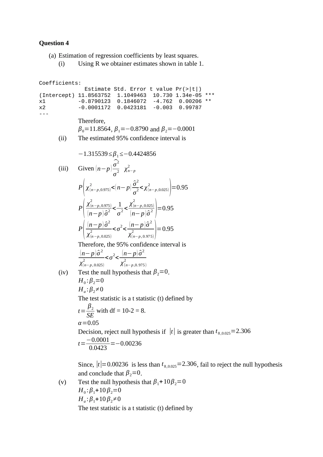
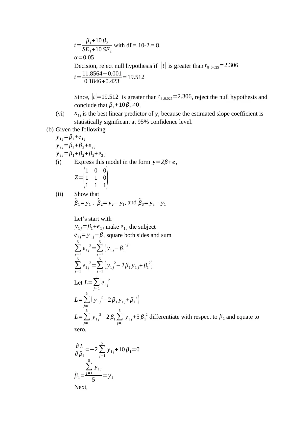
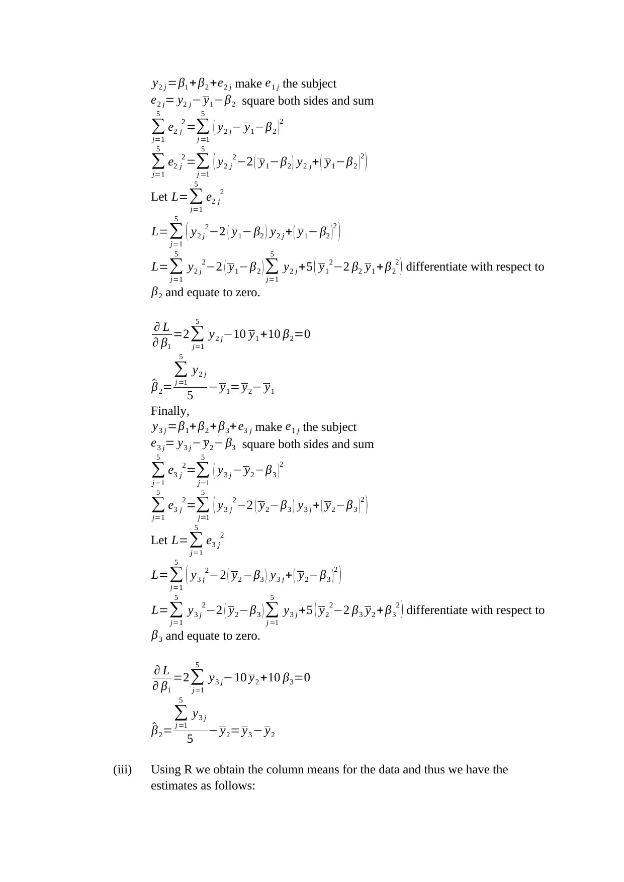
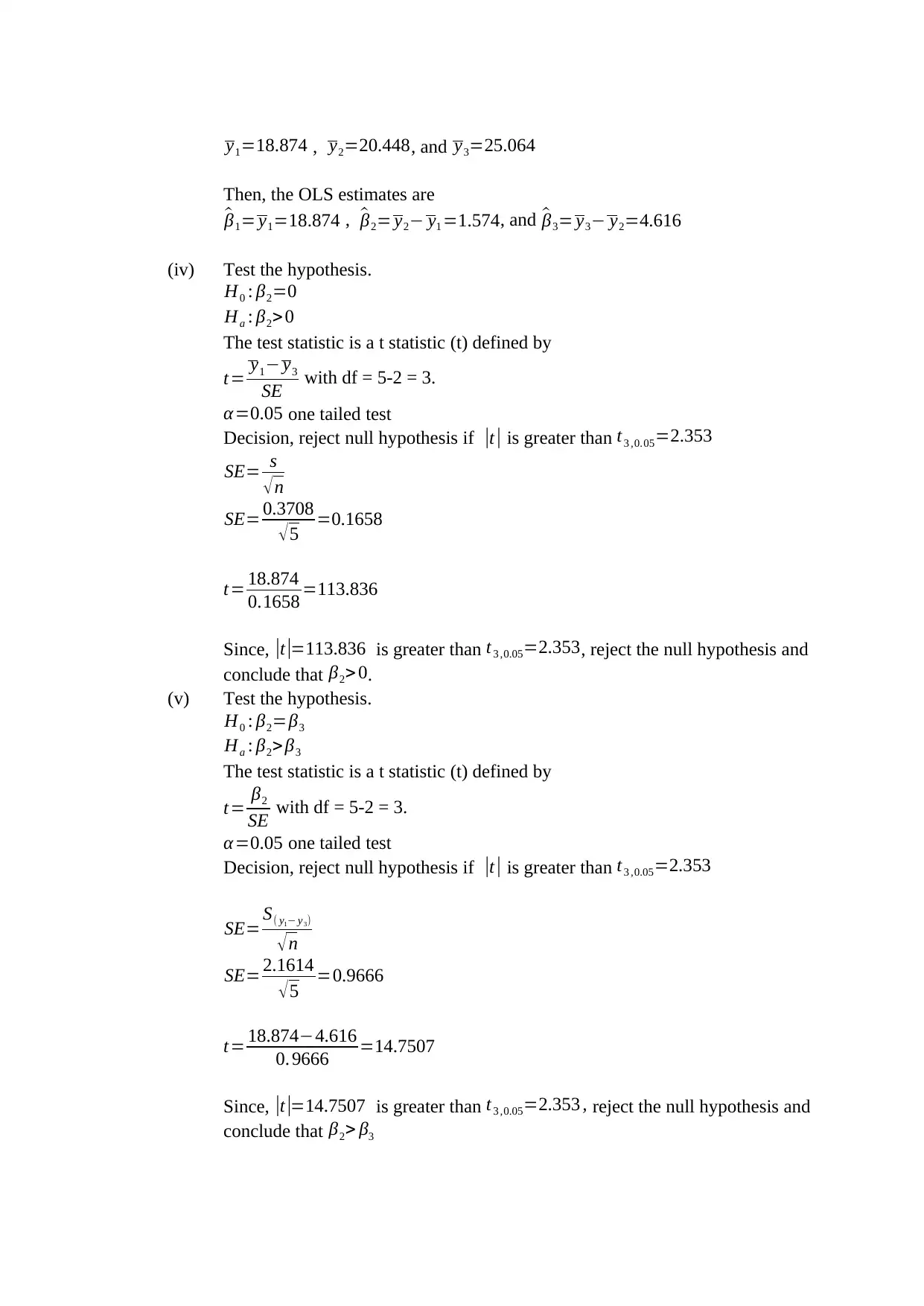
This document provides a comprehensive solution to a linear models coursework assignment, focusing on regression analysis and hypothesis testing. It includes the estimation of regression coefficients using the least squares method, confidence interval calculations, and hypothesis testing for various null hypotheses. The solution utilizes R programming to obtain estimates and statistical summaries, including t-statistics and p-values. The document covers both simple and multiple linear regression models, model fitting, residual analysis, and the interpretation of results. It also explores model transformations and comparisons based on R-squared values, providing a detailed analysis of the statistical concepts and practical applications within the context of the coursework.

Question 4
(a) Estimation of regression coefficients by least squares.
(i) Using R we obtainer estimates shown in table 1.
Coefficients:
Estimate Std. Error t value Pr(>|t|)
(Intercept) 11.8563752 1.1049463 10.730 1.34e-05 ***
x1 -0.8790123 0.1846072 -4.762 0.00206 **
x2 -0.0001172 0.0423181 -0.003 0.99787
---
Therefore,
β0=11.8564, β1=−0.8790 and β2=−0.0001
(ii) The estimated 95% confidence interval is
−1.315539 ≤ β1 ≤−0.4424856
(iii) Given ( n−p ) ^σ 2
σ 2 χn− p
2
P ( χ(n− p ,0.975)
2 < ( n− p ) ^σ2
σ2 < χ(n− p ,0.025)
2
)=0.95
P ( χ(n −p , 0.975)
2
( n−p ) ^σ2 < 1
σ 2 < χ(n− p , 0.025)
2
( n− p ) ^σ 2 )=0.95
P ( ( n−p ) ^σ2
χ(n −p , 0.025)
2 < σ2 < ( n− p ) ^σ 2
χ(n− p , 0.97 5)
2 )=0.95
Therefore, the 95% confidence interval is
( n− p ) ^σ 2
χ(n− p , 0.025)
2 < σ2< ( n− p ) ^σ2
χ(n− p ,0. 975 )
2
(iv) Test the null hypothesis that β2=0.
H0 : β2=0
Ha : β2 ≠ 0
The test statistic is a t statistic (t) defined by
t= β2
SE with df = 10-2 = 8.
α=0.05
Decision, reject null hypothesis if |t | is greater than t8 ,0.025=2.306
t=−0.0001
0.0423 =−0.00236
Since, |t |=0.00236 is less than t8 ,0.025=2.306, fail to reject the null hypothesis
and conclude that β2=0.
(v) Test the null hypothesis that β1+10 β2=0
H0 : β1+10 β2=0
Ha : β1+10 β2 ≠ 0
The test statistic is a t statistic (t) defined by

t= β1+10 β2
SE1+10 SE2
with df = 10-2 = 8.
α=0.05
Decision, reject null hypothesis if |t | is greater than t8 ,0.025=2.306
t= 11.8564−0.001
0.1846+0.423 =19.512
Since, |t |=19.512 is greater than t8 ,0.025=2.306, reject the null hypothesis and
conclude that β1+ 10 β2 ≠0.
(vi) x1 i is the best linear predictor of y, because the estimated slope coefficient is
statistically significant at 95% confidence level.
(b) Given the following
y1 j =β1 +e1 j
y2 j =β1 + β2 +e2 j
y3 j =β1+ β2 + β3+ e3 j
(i) Express this model in the form y=Zβ+e ,
Z=
(1 0 0
1 1 0
1 1 1)
(ii) Show that
^β1= y1 , ^β2= y2− y1, and ^β3= y3− y1
Let’s start with
y1 j =β1 +e1 j make e1 j the subject
e1 j= y1 j−β1 square both sides and sum
∑
j=1
5
e1 j
2 =∑
j =1
5
( y1 j− β1 )2
∑
j=1
5
e1 j
2 =∑
j =1
5
( y1 j
2−2 β1 y1 j+ β1
2 )
Let L=∑
j=1
5
e1 j
2
L=∑
j=1
5
( y1 j
2−2 β1 y1 j + β1
2 )
L=∑
j=1
5
y1 j
2−2 β1 ∑
j=1
5
y1 j +5 β1
2 differentiate with respect to β1 and equate to
zero.
∂ L
∂ β1
=−2 ∑
j=1
5
y1 j +10 β1=0
^β1=
∑
j =1
5
y1 j
5 = y1
Next,

y2 j =β1 + β2 +e2 j make e1 j the subject
e2 j= y2 j− y1−β2 square both sides and sum
∑
j=1
5
e2 j
2 =∑
j =1
5
( y2 j− y1−β2 )2
∑
j=1
5
e2 j
2 =∑
j =1
5
( y2 j
2−2 ( y1−β2 ) y2 j+ ( y1−β2 )2
)
Let L=∑
j=1
5
e2 j
2
L=∑
j=1
5
( y2 j
2−2 ( y1− β2 ) y2 j + ( y1− β2 ) 2
)
L=∑
j=1
5
y2 j
2−2 ( y1−β2 )∑
j=1
5
y2 j +5 ( y1
2−2 β2 y1 + β2
2 ) differentiate with respect to
β2 and equate to zero.
∂ L
∂ β1
=2∑
j=1
5
y2 j−10 y1 +10 β2=0
^β2=
∑
j =1
5
y2 j
5 − y1= y2− y1
Finally,
y3 j =β1+ β2 + β3+ e3 j make e1 j the subject
e3 j= y3 j− y2− β3 square both sides and sum
∑
j=1
5
e3 j
2=∑
j=1
5
( y3 j − y2−β3 )2
∑
j=1
5
e3 j
2=∑
j=1
5
( y3 j
2−2 ( y2−β3 ) y3 j + ( y2−β3 )2
)
Let L=∑
j=1
5
e3 j
2
L=∑
j=1
5
( y3 j
2−2 ( y2 −β3 ) y3 j + ( y2−β3 )2
)
L=∑
j=1
5
y3 j
2−2 ( y2−β3 ) ∑
j =1
5
y3 j +5 ( y2
2−2 β3 y2 +β3
2 ) differentiate with respect to
β3 and equate to zero.
∂ L
∂ β1
=2∑
j=1
5
y3 j−10 y2 +10 β3=0
^β2=
∑
j =1
5
y3 j
5 − y2= y3 − y2
(iii) Using R we obtain the column means for the data and thus we have the
estimates as follows:

y1=18.874 , y2=20.448, and y3=25.064
Then, the OLS estimates are
^β1= y1=18.874 , ^β2= y2− y1 =1.574, and ^β3= y3− y2=4.616
(iv) Test the hypothesis.
H0 : β2=0
Ha : β2> 0
The test statistic is a t statistic (t) defined by
t= y1− y3
SE with df = 5-2 = 3.
α=0.05 one tailed test
Decision, reject null hypothesis if |t | is greater than t3 ,0.05=2.353
SE= s
√n
SE= 0.3708
√5 =0.1658
t= 18.874
0.1658 =113.836
Since, |t |=113.836 is greater than t3 ,0.05=2.353, reject the null hypothesis and
conclude that β2> 0.
(v) Test the hypothesis.
H0 : β2=β3
Ha : β2> β3
The test statistic is a t statistic (t) defined by
t= β2
SE with df = 5-2 = 3.
α=0.05 one tailed test
Decision, reject null hypothesis if |t | is greater than t3 ,0.05=2.353
SE= S( y1− y3)
√n
SE= 2.1614
√5 =0.9666
t= 18.874−4.616
0. 9666 =14.7507
Since, |t |=14.7507 is greater than t3 ,0.05=2.353 , reject the null hypothesis and
conclude that β2> β3

Question 5
(a) Given the model yi=β0 + β1 xi +ei we fit this model using the data given
(i) The estimated model is
Call:
lm(formula = y ~ x, data = coursework4)
Residuals:
Min 1Q Median 3Q Max
-61.297 -25.277 -3.865 8.724 290.438
Coefficients:
Estimate Std. Error t value Pr(>|t|)
(Intercept) -18.429 9.814 -1.878 0.0634 .
x 9.344 1.720 5.431 4.07e-07 ***
---
Signif. codes: 0 ‘***’ 0.001 ‘**’ 0.01 ‘*’ 0.05 ‘.’ 0.1 ‘ ’ 1
Residual standard error: 51.39 on 98 degrees of freedom
Multiple R-squared: 0.2314, Adjusted R-squared: 0.2235
F-statistic: 29.5 on 1 and 98 DF, p-value: 4.072e-07
(ii) The figure 1 shows the scatter plot
(iii) The hypothesis to test as
H0 : β0=β1
Ha : β0 ≠ β1
The test statistic is F statistic given in the summary of the fit.
Since, F1, 98=29.5 , p <0.00, We reject the null hypothesis at 95% since p-value
is less than α =0.05.
(iv) The four in one figure below shows the residual plot for the fitted model

The Q-Q plot shows that majority of the points are along the diagonal line.
Therefore, assumption of normality of the residuals is satisfied.
(b) Given the model
yi=α eβ xi
Transform the equation by taking log both sides
ln ( yi)=ln (α )+ β xi
Let β0=ln (α ) , ~yi=ln ( yi). Then the regression equation becomes
~yi =β0+ β xi+ ei
(i) We use R to estimate the model and the estimates are shown below
Call:
lm(formula = y1 ~ x, data = coursework4)
Residuals:
Min 1Q Median 3Q Max
-2.76708 -0.75478 0.05246 0.78888 2.28723
Coefficients:
Estimate Std. Error t value Pr(>|t|)
(Intercept) -0.40690 0.21157 -1.923 0.0573 .
x 0.46480 0.03709 12.533 <2e-16 ***
---
Signif. codes: 0 ‘***’ 0.001 ‘**’ 0.01 ‘*’ 0.05 ‘.’ 0.1 ‘ ’ 1
Residual standard error: 1.108 on 98 degrees of freedom
Multiple R-squared: 0.6158, Adjusted R-squared: 0.6119
F-statistic: 157.1 on 1 and 98 DF, p-value: < 2.2e-16
(ii) Figure 2 shows the scatter plot

(iii) The hypothesis to test is
H0 : β0=β
Ha : β0 ≠ β
The test statistic is F statistic given in the summary of the fit.
Since, F1, 98=157.1 , p< 0.00, We reject the null hypothesis at 95% since p-
value is less than α =0.05.
(v) The four in one figure below shows the residual plot for the fitted model
The Q-Q plot shows that majority of the points are along the diagonal line.
Therefore, assumption of normality of the residuals is satisfied.
The first model has R-square of 0.2314 while the second model has R-square
of 0.6158. Therefore, the second model is better than a the 1st model.