BUSN7051 Assignment 1 - Formulation and Solution of Linear Programs

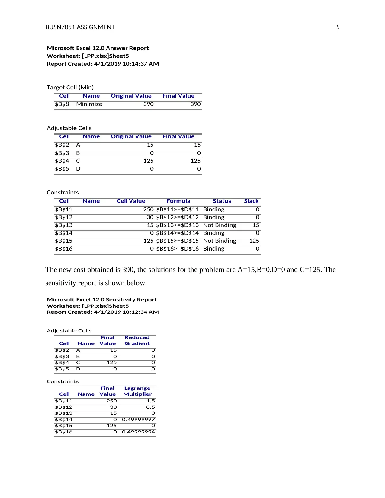
This document presents a comprehensive solution to BUSN7051 Assignment 1, focusing on linear programming techniques. The solution includes the formulation of a linear programming problem, determining variables, and defining the objective function to maximize production output. It outlines constraints related to machine processing times, initial stock levels, and demand forecasts for two products, X and Y. The solution utilizes the Iso-profit line method to find the optimal solution, followed by a graphical representation. The document further addresses a second linear programming problem, including minimizing costs and sensitivity analysis using Microsoft Excel. It provides the optimal solution, the minimum cost, and sensitivity reports, as well as a discussion of the impact of changing constraint values. The assignment concludes with a list of references, including key texts on operations management.

BUSN7051 ASSIGNMENT 1
Australian National University
BUSN7051 ASSIGNMENT
Student Name

BUSN7051 ASSIGNMENT 2
2. Formulation of the problem that will aid in deciding the quantity of each product to make in
the present week.
(a) Determining variables that are not known.
Quantity of X units produced in the present week week=x
Quantity of Y units produced in the current week=y
(b) Formulating the objective function for the program
The organizations aim is to maximize a combine sum of units’ production for product
X and those of Y. The objective function Z is thus:
To maximize the number of units left in stock at the end of the week
(x+30-75)+(y+90-95)=x+y-50
(c) The constraint of the Linear programming problem are:
50x + 24y ≤ 2400
30x + 33y ≤ 2100
x≥ (75 – 30)
x≥ 45
The amount of X produced ≥ demand (75) - initial stock quantity is 30, which
ensures we meet demand
y≥ 95 - 90
y ≥ 5, The amount units of Y produced ≥ demand (95) – initial value of stock is
(90), This will ensure the company demand is met.
(d) We utilize the Iso-profit profit line method to solve the linear program developed
above. To maximize our objective function, we draw the Iso profit line
which will enable us find the maximum value of the objective function.
Variables
x 45
y 6.25
Objective
Maximize 1.25
Constraints inequality
1 2400 <= 2400
2 1556.25 <= 2100
3 45 >= 45
4 6.25 >= 5
The point that maximizes x+y-50 is (45,6.25),
The solution to the linear program is 45+6.25-50=1.25.

BUSN7051 ASSIGNMENT 3
The graphical representation from desmos graphs is as below
3. (a). Minimize P=A+2B+3C+4D
Subject to
B+2C+2D≥100
2A+D≥30
A,B,C,D≥0

BUSN7051 ASSIGNMENT 4
Variables
A 15
B 0
C 50
D 0
Objective
Minimize 165
Constraints
1 100 >= 100
2 30 >= 30
3 15 >= 0
4 0 >= 0
5 50 >= 0
6 0 >= 0
(b)The optimal solution of the Linear programming problem is A=15,B=0, C=50, D=0.
(c).The minimum cost is 165.
The Sensitivity analysis report
Microsoft Excel 12.0 Sensitivity Report
Worksheet: [LPP.xlsx]Sheet3
Report Created: 4/1/2019 10:09:01 AM
Adjustable Cells
Final Reduced
Cell Name Value Gradient
$B$2 A 15 0
$B$3 B 0 0
$B$4 C 50 0
$B$5 D 0 0
Constraints
Final Lagrange
Cell Name Value Multiplier
$B$11 100 1.5
$B$12 30 0.5
$B$13 15 0
$B$14 0 0.500000328
$B$15 50 0
$B$16 0 0.5
(d). If the value of the minimal requirement of the first constraint increased from 100 to 250 and
the problem is run in solver, the output is shown below.

BUSN7051 ASSIGNMENT 5
Microsoft Excel 12.0 Answer Report
Worksheet: [LPP.xlsx]Sheet5
Report Created: 4/1/2019 10:14:37 AM
Target Cell (Min)
Cell Name Original Value Final Value
$B$8 Minimize 390 390
Adjustable Cells
Cell Name Original Value Final Value
$B$2 A 15 15
$B$3 B 0 0
$B$4 C 125 125
$B$5 D 0 0
Constraints
Cell Name Cell Value Formula Status Slack
$B$11 250 $B$11>=$D$11 Binding 0
$B$12 30 $B$12>=$D$12 Binding 0
$B$13 15 $B$13>=$D$13 Not Binding 15
$B$14 0 $B$14>=$D$14 Binding 0
$B$15 125 $B$15>=$D$15 Not Binding 125
$B$16 0 $B$16>=$D$16 Binding 0
The new cost obtained is 390, the solutions for the problem are A=15,B=0,D=0 and C=125. The
sensitivity report is shown below.
Microsoft Excel 12.0 Sensitivity Report
Worksheet: [LPP.xlsx]Sheet5
Report Created: 4/1/2019 10:12:34 AM
Adjustable Cells
Final Reduced
Cell Name Value Gradient
$B$2 A 15 0
$B$3 B 0 0
$B$4 C 125 0
$B$5 D 0 0
Constraints
Final Lagrange
Cell Name Value Multiplier
$B$11 250 1.5
$B$12 30 0.5
$B$13 15 0
$B$14 0 0.49999997
$B$15 125 0
$B$16 0 0.49999994

BUSN7051 ASSIGNMENT 6
References
Heizer, J. and Render, B. (2013). Operations Management, Global Edition. Edinburgh: Pearson
Education.
Hill, A. and Hill, T. (2012). Operations management. Houndmills, Basingstoke, Hampshire:
Palgrave Macmillan.
Stevenson, W. (2012). Operations management. New York, N.Y.: McGraw-Hill/Irwin.